Introduction
Xnec2c is a GTK3-based Graphical version of nec2c, my translation to the C language of NEC2, the FORTRAN Numerical Electromagnetics Code commonly used for antenna simulation and analysis. The original nec2c is a non-interactive command-line application that reads standard NEC2 input files and produces an output file with data requested by "commands" in the input file. In contrast xnec2c is a GUI interactive application that (in its current form) reads NEC2 input files but presents output data in graphical form, e.g. as wire frame drawings of the radiation pattern or near E/H field, graphs of maximum gain, input impedance, VSWR etc against frequency and simple rendering of the antenna structure, including color code representation of currents or charge densities. These results are only calculated and drawn on user demand via menu items or buttons, e.g. xnec2c is interactive and does not execute NEC2 "commands" in batch style as the original does. Printing of results to an output file has been removed starting from v1.0, since xnec2c works in a way that does not allow printing compatible with the NEC2 format. If printing to file is needed then it is better to use the original NEC2 program, to avoid bugs that may still be lurking in the C translation.
Xnec2c now has a built-in editor for NEC2 input files which can be used to edit geometry or command "card" data. This basic editor displays comment, geometry and command cards in tree views where individual rows, each representing a card, can have their cells edited directly for "raw" entry of data. More useful are pop-up "editor" windows that open when appropriate buttons are clicked or when a selected row is right-clicked with the mouse. These editors allow easier, more convenient entry and editing of individual rows, with no need for detailed knowledge of "card" formats. When editing is completed, the contents of the nec2 editor can be saved in a NEC2-compatible input file which can then be re-loaded by xnec2c for execution.
Features
Multi-threading operation on SMP machines
Since v1.0, xnec2c can run multi-threaded (by forking) on
SMP machines, when executing a frequency loop. Multi-threading is
enabled by using the -j <n> option, where n is the number of
processors in a SMP machine. xnec2c will spawn n child processes,
to which it will delegate calculation of frequency-dependent data
for each frequency step. Thus data related to n frequency steps
will be calculated concurrently and passed on the the parent
process by pipes, to be further processed for graphical display.
Child processes are spawned before GTK is initialized and started
so that only the parent process is tied to the GUI interface. Thus
there are n+1 processes running when the -j option is used and
execution is faster by slightly less than n times.
On-demand Calculation
Since xnec2c collects data to be displayed in buffers directly from the functions that produce them, there is no need to produce and parse an output file and no need to re-run the program when certain input data (currently the frequency) is changed or when different output data (gain, near-fields, input impedance etc) is required. The frequency can be changed either from spin buttons in the Main and Radiation Pattern windows or by clicking on the Frequency Data window's graph drawing area. The frequency corresponding to the pointer position will then be used to re-calculate whatever data is on display.
Built-in NEC2 input file editor
Xnec2c has a built-in editor for NEC2 input files. Data in NEC2 "cards" can be entered or edited either directly in the main editor window (tree view) or in more convenient dedicated editors for each type of card. Edited data can be saved to a NEC2 input file and reloaded for execution so that the edit-execute-display cycle is quicker and more convenient.
Accelerated Linear Algebra Support
Support for accelerated libraries was added in v4.3. Accelerated math libraries such as ATLAS, OpenBLAS and Intel MKL can speed up xnec2c EM simulations if available on your platform. Library detection details are available in the terminal. See for more information. Accelerated operation is optional, it will fall back to the original NEC2 algorithms if necessary. Accelerated library support has been tested on Ubuntu , Debian, CentOS/RHEL, and VOID Linux. Generally speaking, if you can install the requisite libraries, it will be detected. If libraries are not detected on your OS then please open a bug report.
Interactive Operation
Xnec2c is interactive in its operation, e.g. when started it just
shows its Main window in a "blank" state, indicating that no valid
input data has been read in yet. The NEC2-type input file can be
specified at start-up in the command line optionally with the -i
option or it can be opened from the file selection dialog that
appears via the menu of the Main window. Once a valid input file is opened,
all the normal widgets in the Main window
appear so as to allow proper operation. The NEC2 "commands" in the
input file are read in but not executed, until a request is issued
by the user via buttons or menus in the appropriate windows.
User Interface
In its current form, xnec2c has three windows for the graphical display of output data: When started without an input file specified optionally by the-i <input-file> option, the
Main window opens with most of the button
and menu widgets hidden. When a valid input file is opened, all the
hidden widgets are shown and the structure is drawn in the Main window's drawing area widget. From the
View menu, the Radiation
Pattern and Frequency Related
data display windows can be opened, to draw either the Gain
pattern or the Near E/H fields or Frequency-related Data like Input
Impedance, VSWR, Max gain, F/B Ratio, Gain in the Viewer's
direction etc. Both the Main window and
the Radiation Pattern window have
buttons to select fixed viewing angles of the structure or the
radiation pattern, as well as spin buttons to input specific
viewing angles.
When built with OpenGL support, both windows use a hardware-accelerated
3D renderer with configurable anti-aliasing, transparency, and
draw-style options; see OpenGL Rendering.
Noise Temperature Visualization
The Radiation Pattern window can render each solid-angle cell of the pattern by its gain-weighted brightness temperature (K/sr) under a selectable RF noise environment, showing where noise enters the antenna. Three independent selectors—sky model, earth model, and interpolation method—determine the Tsky and Tearth values assigned to each hemisphere. An elevation control virtually rotates the antenna pattern to the desired observation elevation. The Frequency Plots window displays Tant, Ttotal, and G/Tant across the operating band.
Average Power Gain
When the RP card specifies at least two theta and two phi steps,
xnec2c computes the average power gain over the radiation sphere
after each frequency step. The result is printed to the console as a
linear ratio, in dBi, and as a radiation efficiency percentage. An
ideal lossless antenna with complete sphere coverage produces an
average gain of 1.0 (0.0 dBi, 100% efficiency); lower values
indicate resistive or ground losses. This diagnostic is enabled
automatically unless --skip-verify is active.
Color Coding
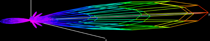
Xnec2c uses color coding to visualize the Current or Charge distribution in the Structure's segments or patches as well as the Gain pattern or the Near E/H field pattern. Color coding is also used to clarify the Graphs of Frequency-related data. A color code strip is shown in the Main and Radiation Pattern windows.
Compilation and Installation
Binary packages are available via Flathub for Linux (thanks to AsciiWolf in issue #29), MacPorts for macOS (thanks to Carl Makin in issue #66), and FreeBSD FRESH ports. Xnec2c is known to build from source on many different platforms including Linux. If you have trouble building on your OS then please open a bug report.
To compile the package, it may be preferable to first run the
included autogen.sh script in the package's top directory, to
produce a fresh build environment. Then the configure script can
be run with optional parameters to override the default settings
and compiler flags, e.g: ./configure --prefix=/usr CFLAGS="-g -O2"
will override the default /usr/local installation prefix and the
-Wall -O2 compiler flags.
Running make in the package's top directory should produce the
executable binary in src/. Running make install will install the
binary into /usr/local/bin by default or under the specified
prefix. It will also install the default configuration file into
the user's home directory. This will have to be edited by the user
as required. There is also this hypertext documentation file which
you can copy to a location of your choice.
No configuration files are needed and the sample input files that were used during development are in the examples directory. Please also read the doc/nec2c.txt file that describes the nec2c application that is used as the basis for xnec2c.
Operation
Command Line Options
Usage: xnec2c [options] [<input-file-name>]
The following arguments write to an output file after the frequency loop
completes. These are useful to combine with --batch; If you wish to specify
filenames to write without --batch mode then enable the or the files you specify on the command line will not be written.
Command Line Notes
<input-file-name>: Specify a NEC2 input file to
be opened at start-up. If the -i option is omitted, xnec2c will
take the last argument to be the input file path name, but will
only open it if it has the .nec extension.
<number of child processes to spawn>: Since v1.0 xnec2c can run multi-threaded on SMP machines. This option specifies the number of child processes to spawn by forking, so that the total number of processes running will be n+1. n should be equal to the number of processors in a SMP machine.
Starting in v4.3, xnec2c always forks at least one job
for better UI responsiveness. If you wish to disable forking for
debug or testing then specify -j0.
Internationalization
Xnec2c supports 42 languages via GNU gettext. The language is
selected automatically from the system locale. To override, set the
LANGUAGE environment variable before launching — for
example, LANGUAGE=de xnec2c for German. If the compiled-in
locale directory is not correct for your installation, set
XNEC2C_LOCALEDIR to point to the directory containing the
LC_MESSAGES trees.
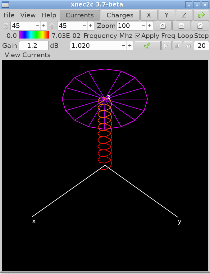
The Main Window
-i option can be used to specify a NEC2 input file:
xnec2c -i ~/nec2/turnstile.nec. Otherwise an input file can
be opened from the Main window's menu o
item. If the input file is valid, xnec2c will render the structure
specified in the Geometry section of the file in the Main window's
drawing area. The background color is black and the structure is
rendered in blue. The excitation points (segments) are rendered in
red, the x, y, z axis in white, loaded segments in yellow,
transmission lines in cyan and two-port networks in magenta. These
default colors are supplied by the active color theme; the current color
projection controls (see Current Color
Projection and Tone Mapping) determine how current and charge map to
color, and the frequency plots carry their own selectable themes.
Once an input file is opened, the structure display can be rotated around the Z axis and tilted about a horizontal axis through the origin. This can be done either by pressing button #1 and dragging the structure with the mouse pointer, clicking the (x), (y), (z), or (d) view button (45° rotation and tilt). The actual value of rotation and tilt is shown in two spin button widgets which can also be used to change the viewing angle.
Starting with v2.1, the structure display can be zoomed in or out by using the mouse wheel or the Zoom controls: spin wheel and the (Ctrl+Plus), (Ctrl+Minus), and (Ctrl+1) buttons and it can also be moved around by dragging with the right mouse button #2.
The current distribution or charge density in the structure can be displayed by clicking the (i) or (v) toggle buttons at the top right of the Main window. The distribution of current or charges is rendered by a color code, red for the maximum value and magenta for zero. The Frequency Loop control buttons can be used to Start, Pause or Reset the loop. There is a bar at the left of the second row of widgets in the Main window, indicating the color coding and the maximum value of the displayed quantity (at its right).
The title in the border of the drawing area widget shows the user-selected function of the display, while the text entry widget at the right of the color code bar shows antenna gain in the Viewer direction, e.g. perpendicular to the Screen. To the right of this the shows the current frequency in MHz for which the current/charge distribution and Viewer gain are calculated and displayed. If the is active, each time the frequency is changed in the spin button, all relevant data on display will be recalculated. If not, clicking the Redo button will initiate recalculation.
Printing of results to an output file has been removed starting from v1.0, since xnec2c works in a way that does not allow printing compatible with the NEC2 format. If printing to file is needed then it is better to use the original NEC2 program, to avoid bugs that may still be lurking in the C translation. Otherwise, it is possible to save the structure drawing to a PNG file by using the (s) or (Ctrl+s) items in the File menu.
Starting with v2.1, xnec2c can save the structure display
as a data file for the gnuplot plotting program. This is done by
using the menu item, to open a file
chooser dialog. If only the stem of the file name is given, xnec2c
will automatically add the .gplot extension. Plotting in gnuplot is
done with the splot <filename> with lines command, although
the plot can be enhanced with some of the style etc commands
available in gnuplot.
The menu allows opening of other output data display
windows and selection of various options:
The menu (r) item opens the Radiation Pattern window so that the Gain
pattern or the Near E/H fields can be calculated and displayed.
The menu (f) item opens the Frequency Data Plots window which allows the
plotting of various frequency-related data against the frequency
range specified in the FR command. It also allows quick selection
of the current frequency and recalculation of data by clicking on
the plots drawing area.
The submenu allows the selection of different
polarizations for which many data items are calculated (e.g. gain,
F/B ratio etc). The selection is global, e.g. it effects all
relevant data that are drawn or displayed in other windows.
The item couples the projection (viewing
angle) parameters of the Structure display in the Main window and
the Gain or E/H field display in the Radiation pattern window so that both move
in step.
The submenu selects how current
flow is depicted on the structure; see
Current Flow Visualization.
The item opens the
Near Field Animation panel.
The item opens the
SY parameter tuning window.
The item opens the
renderer configuration dialog.
The toolbar includes an toggle button that switches between perspective and orthographic projection; see Orthographic Projection. The and spin buttons accept mouse-wheel scrolling in 5° increments and have extended ranges (Rotate 0–720°, Incline ±360°) to allow continuous dragging past the original limits; values wrap automatically at 360° and ±180° respectively. With the OpenGL renderer active, Ctrl+Scroll adjusts the visual thickness of wire segment cylinders (equivalent to the Cylinder Scale slider). Scrolling down past the minimum snaps to line rendering mode, where segments draw as thin lines instead of 3D cylinders; scrolling back up returns to cylinder mode. This does not affect NEC2 model calculations.
The Radiation Pattern window
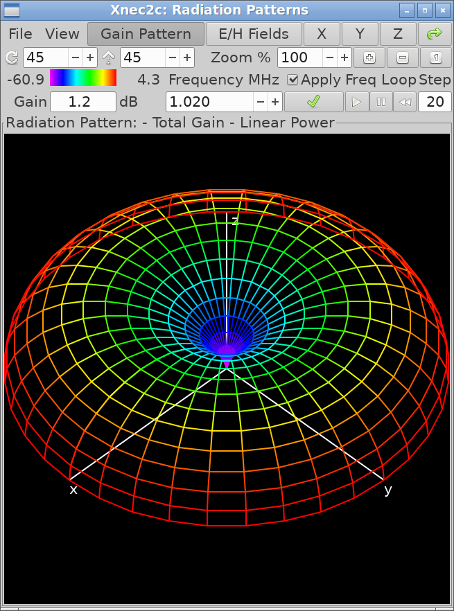
RP) command, the Gain pattern
will be calculated and drawn. The E/H field will be properly drawn
if there are at least two points specified in the NE or NH
commands. The Frequency Loop control buttons at the far right can
be used to Start, Pause and Reset the loop.
The menu, in addition to the check button, provides
submenus for selecting type,
(which includes Noise Temperature modes),
Noise Models,
Draw Style (Surface, Wireframe, or Both),
a toggle for the color legend,
and the data to be drawn. The
selection of polarization type affects the Gain pattern, the
displayed Viewer gain and the value of max and min gain as shown to
the left and right of the color code bar. The selection of gain
scaling only affects the form of the Gain pattern drawing:
is the most realistic, since the distance from
the origin of each point in the gain pattern is proportional to the
radiated power density, as is the color code (red for max gain and
magenta for min gain). A disadvantage of this scaling is the
inadequate representation of side lobes since they are usually
significantly weaker than the main beam. is
better in this respect since the position of points in the gain
pattern is proportional to Electric field strength and hence
follows a square root law. follows a form of
logarithmic scaling suggested by the American Radio Relay League,
e.g. exp(0.058267 × gain) where gain is in dB10. Finally
follows a logarithmic scale with a median of
40 dB.
When a Near Field (NE or NH) command is included
in the input file, clicking the (f) button
produces a drawing of the near Electric and/or Magnetic fields. By
selecting the menu item the
Poynting vector is also drawn. These fields are depicted by lines
of fixed length in the direction of the relevant (E/H/Poynting)
vector at each point in the drawing. The field strength is depicted
by the color of the lines as using the line length for this purpose
makes most lines too small to be useful. The drawing of the Near E
or H Fields can be enabled or disabled by the and
menu items.

The menu item (also available from in the Main window) opens the Near Field Animation panel, which drives the phase animation and the current, charge, and near-field color mapping. See Near Field Animation and Color Mapping for its controls.
The sub-menu allows the selection of drawing either the value or a "time-frozen" snapshot of the instantaneous value of the total Near Field E/H vectors. The Snapshot values are calculated as the vector sum of the X, Y, Z components of the E/H field and the Peak values are calculated using the formula NEC4 uses to print the Peak field values.
The menu item enables the drawing of the structure in the radiation pattern drawing area when the Near Field pattern is selected for drawing. This makes it easier to understand the scale and extend of the Near Field patterns around the structure. The color scheme for the structure becomes white when Overlay is enabled, unless it is overridden by either the Current or Charge distribution being enabled by the relevant buttons in the Main window. With the OpenGL renderer, Shift+Scroll scales the overlay structure relative to the radiation pattern (gain view only; inactive in near-field mode), and Ctrl+Scroll adjusts wire cylinder thickness as in the Main window.
In the second row of widgets, the bar shows either the max and min values of Gain in the radiation pattern or the maximum value of the field strength in the near E/H field pattern. (Of course only one value can be shown, the precedence being E field, H field or Poynting field strength, depending on which of these is enabled in the sub menu). The widget at the right of the color bar shows gain in the direction of the viewer (perpendicular to screen), while the following it shows the current frequency in MHz for which data is displayed. It can also be used to enter a new frequency in the same manner as in the Main window. The enables re-calculation and display of data when the frequency value changes, while the button to its right causes same when clicked by the user, but only if a new frequency has been entered.
The Gain pattern draw style is selectable from : renders a filled triangulated mesh, draws colored line segments, and overlays wireframe on a dimmed surface. In all modes each element is colored according to the average value of gain associated with its vertices. The pattern can be "dragged" with the mouse pointer to rotate or tilt it and it can also be positioned using either the (x), (y), (z), or (d) buttons. The and spin buttons can also be used to accurately position the Gain pattern in the window. The in the drawing area's frame gives information on what is on display and also the type of polarization or gain scaling.
Starting with version 2.1, the radiation pattern display can be zoomed in or out by using the mouse wheel or the Zoom controls ( spin wheel and the (Ctrl+Plus), (Ctrl+Minus), and (Ctrl+1) buttons) and it can also be moved around by dragging with the right mouse button #2.
Both the Gain and Near Field patterns can be saved as PNG image files by using the menu (s) or menu (Ctrl+s) items. The Save option will save the drawings with a suitable default file name which includes a serial number, so that consecutive Saves do not overwrite files.
Starting with v2.1, xnec2c can save the radiation pattern
and near E/H field display as a data file for the gnuplot
plotting program. This is done by using the menu item, to open a file chooser dialog. If only the
stem of the filename is given, xnec2c will automatically add the
.gplot extension. Plotting in gnuplot is done with the splot
<filename> with lines command, although the plot can be
enhanced with some of the style etc commands available in
gnuplot.
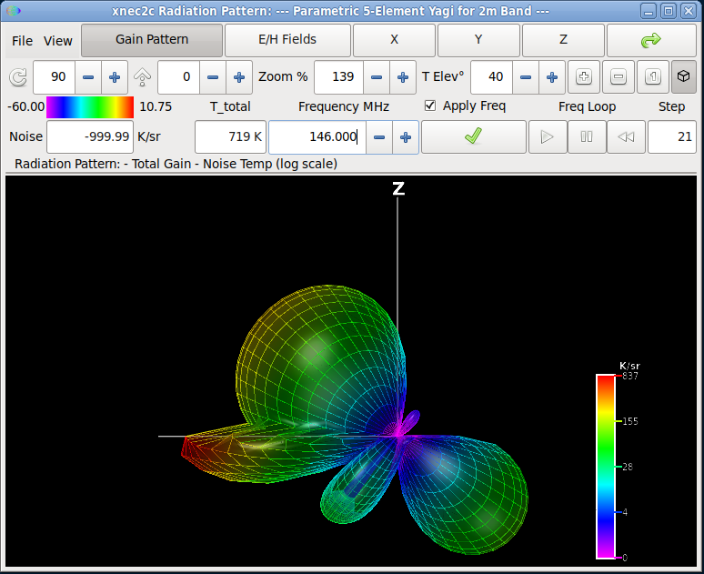
Noise Temperature Display
Two additional entries in the submenu render the radiation pattern by noise temperature rather than gain magnitude. colors each solid-angle cell by its gain-weighted brightness temperature in K/sr (Kelvin per steradian), using a linear scale. Cells receiving high brightness temperature from the environment appear at the red end of the color bar; those contributing little noise appear at the magenta end. applies logarithmic compression, revealing low-level sidelobe contributions that the linear mapping compresses into a narrow color band.
The color legend adapts to show the K/sr range of the current pattern rather than dB gain values. Relative dB marks along the legend are suppressed, since they have no meaning in temperature units. The gain readout below the color bar likewise displays K/sr. To verify correct operation, observe that the highest-temperature cell corresponds to the direction facing the warmer hemisphere (earth, when elevation is 0° or positive) with the strongest pattern gain in that direction.
Noise temperature computation requires gain data over the full sphere. Xnec2c displays a one-time warning when it detects conditions that compromise the result. Two such conditions exist: a ground-plane model provides gain data for only the upper hemisphere, leaving the lower hemisphere—where earth noise would normally dominate—without computed values; and a beam maximum that lies significantly off the model's forward axis can distort the G/Tant figure of merit, since the reference gain no longer represents the intended receive direction.
Noise Models
The submenu controls which brightness temperatures are assigned to the sky and earth hemispheres. Three independent selectors appear in the menu, separated by headings: Sky Model, Earth Model, and Interpolation. Any sky model can be combined with any earth model.
Sky and earth temperatures describe physically distinct emission sources. Tsky is dominated by galactic synchrotron radiation—diffuse radio emission from the Milky Way—which decreases steeply with frequency (roughly as f−2.75). Tearth is dominated by man-made electrical noise from power lines, motors, and electronics, which also decreases with frequency but at a rate that depends on the density of the local built environment. The two quantities are independent: a rural site under galactic center sees low earth noise but high sky noise, while a city rooftop pointed at the galactic pole sees the opposite. Selecting sky and earth models independently reflects this physical reality.
Sky Models
| Model | Bands | Purpose |
|---|---|---|
| G4CQM Min Quiet (pre-2016) | 50, 144, 222, 432, 1296 | Minimum quiet-sky temperatures from the G4CQM reference data used in VK3UM’s EME Calculator. Represents the coldest sky an antenna can point at, away from the galactic plane. Use for best-case EME system noise budgets. |
| VK3UM Min Quiet (pre-2016) | 50, 144, 220, 432, 900, 1296 | Minimum quiet-sky values from VK3UM’s Radio Path Calculator. Similar to G4CQM but includes 220 and 900 MHz bands. Useful when those intermediate frequencies are needed. |
| VE7BQH Base Ref (pre-2018) | 50, 144, 432 | Frozen pre-2018 normalization values (1700, 200, 20 K). Historical reference for comparing against older VE7BQH table editions. Superseded by DG7YBN Galactic Avg for current work. |
| Galactic P.372 (2022) | continuous | Galactic noise computed from ITU-R P.372-16 equations 13 and 14. Below 100 MHz the log-linear man-made noise formula applies (Fam = 52 − 23·log10(f)); above 100 MHz a power-law extrapolation (T ∝ f−2.75) plus the 2.7 K cosmic microwave background. This is the mathematical all-sky average, which runs higher than practical antenna measurements above 100 MHz (e.g., 425 K at 144 MHz versus 290 K for DG7YBN). Select this for theoretical analysis or when no tabulated data covers the operating frequency. |
| DG7YBN Galactic Avg (2025) | 50, 144, 432 | Average galactic background as used in the DG7YBN/VE7BQH antenna comparison tables. Select this to reproduce published VE7BQH G/T values. Values represent a practical average over the sky as seen by a directional antenna, lower than the mathematical all-sky average at VHF. |
| Synth Practical Avg (2026) | 50, 100, 112.5, 137.5, 144, 220, 222, 250, 401, 402.5, 408, 432, 500, 761, 900, 1000, 1296 | Synthesized practical-average galactic sky derived from cross-referencing DG7YBN, G4CQM, and P.372 data. Follows the galactic formula closely below 144 MHz, then tracks practical antenna measurements at higher frequencies. The broadest-coverage sky model for general antenna comparison. |
| Synth Min Quiet (2026) | 50, 100, 112.5, 137.5, 144, 220, 222, 250, 401, 402.5, 408, 432, 500, 761, 900, 1000, 1296 | Synthesized minimum quiet sky. Coldest achievable sky across the full VHF/UHF range. Use for best-case system noise analysis with fine frequency resolution. |
Earth Models
| Model | Bands | Purpose |
|---|---|---|
| ITU-R Business (1974) | continuous | High urban and industrial noise computed from the ITU-R P.372 man-made noise formula (Fam = 76.8 − 27.7·log10(f)). Continuous across 0.3–250 MHz. At higher frequencies the formula drops below 290 K and is clamped to the ambient thermal floor. |
| ITU-R Residential (1974) | continuous | Suburban residential noise computed from formula (Fam = 72.5 − 27.7·log10(f)). Floor activates around 323 MHz. |
| ITU-R Rural (1974) | continuous | Low-density rural noise computed from formula (Fam = 67.2 − 27.7·log10(f)). Floor activates around 208 MHz. |
| ITU-R Quiet Rural (1974) | continuous | Minimal man-made noise computed from formula (Fam = 53.6 − 28.6·log10(f)). Approaches the 290 K thermal floor above approximately 59 MHz. Select this for remote sites far from electrical infrastructure, such as EME or radio astronomy installations. |
| G4CQM Mixed (pre-2016) | 50, 144, 222, 432, 1296 | Mixed-use environment from the G4CQM tabulated reference data. Independent of the DG7YBN and ITU classification schemes. Values are moderate, between rural and residential. |
| VE7BQH Base Ref (pre-2018) | 50, 144, 432 | Frozen pre-2018 tabulated earth values (9000, 1000, 350 K). Historical reference for older VE7BQH table comparison. Superseded by the DG7YBN earth models for current work. |
| DG7YBN Rural (2025) | 50, 144, 432 | Low man-made noise from the DG7YBN/VE7BQH tabulated data. Select this with DG7YBN Galactic Avg sky to reproduce published VE7BQH Rural G/T values. |
| DG7YBN Residential (2025) | 50, 144, 432 | Moderate man-made noise from tabulated data. The default pairing with DG7YBN Galactic Avg for standard VE7BQH table comparison. Represents a typical suburban location. |
| DG7YBN City (2025) | 50, 144, 432 | High man-made noise from tabulated data. Urban and industrial environments with dense electrical infrastructure. |
Interpolation Method
The interpolation selector governs how table-based models (those with discrete frequency anchors) resolve temperatures at arbitrary frequencies. It does not apply to formula-based models (ITU-R earth, Galactic sky), which compute values directly from their equations.
| Method | Behavior |
|---|---|
| Snap | Use the temperature from the nearest tabulated frequency. No values are fabricated between bands. This is the correct method for DG7YBN and VE7BQH models, whose per-band values are independent community estimates rather than samples from a continuous curve. Interpolating between them would assert a smooth relationship that was never claimed by the source data. |
| Interpolate | Log-log interpolation between adjacent table anchors, clamped to the nearest anchor outside the table range. Appropriate for models with many anchor points (G4CQM, VK3UM, Synth) where smooth inter-band coverage is desired. When the operating frequency falls between two anchors, the temperature is computed by linear interpolation in log-frequency/log-temperature space. |
When the sky or earth model changes, the interpolation selector automatically switches to the method that model was designed for. The user can override this afterward. For example, selecting DG7YBN Galactic Avg sets Interpolate as the default; the user can switch to Snap to see the nearest-band value instead.

Choosing Models
To reproduce published VE7BQH antenna comparison table values, select DG7YBN Galactic Avg sky with the appropriate DG7YBN earth model (Rural, Residential, or City). For broadband antenna development where smooth frequency coverage matters, Synth Practical Avg sky with an ITU-R earth model provides continuous Tsky and Tearth across the full VHF/UHF range. For EME system noise budgets, pair a minimum quiet sky model (G4CQM, VK3UM, or Synth Min Quiet) with ITU-R Quiet Rural earth to represent the coldest achievable environment. The Galactic (P.372) sky model is useful for theoretical analysis at frequencies outside the tabulated ranges or for comparing practical antenna measurements against the mathematical all-sky prediction.
The ITU-R formula can yield Tearth values below the physical ambient temperature at higher VHF frequencies in quieter environments; xnec2c clamps Tearth to a 290 K floor in these cases, since no terrestrial environment can be colder than its physical surroundings.
All three selections are persisted in the configuration file and restored on next startup.
Elevation Offset
The spin button in the toolbar sets the observation elevation angle. The range is −90° to +90°. The antenna pattern is virtually rotated so that its maximum-gain direction points at the specified elevation above the horizontal plane. The sky/earth boundary remains fixed at the geometric horizon: cells facing upward after rotation see Tsky, cells facing downward see Tearth. In the 3D display the pattern visually tilts upward by the elevation amount while the ground stays at the bottom. Positive values model an antenna pointed above the horizon where more of the pattern sees cold sky; negative values point the antenna downward, increasing earth hemisphere coverage.
This setting affects both the 3D noise temperature coloring and the scalar Tant computation. To confirm the relationship, set elevation to +90° and observe that Tant approaches Tsky (the entire pattern faces sky). At −90° it approaches Tearth. At exactly 0°, an isotropic antenna produces Tant = (Tsky + Tearth) / 2, since the two hemispheres subtend equal solid angle and every cell has identical gain.
The elevation value is persisted in the configuration file.
Understanding Antenna Temperature
Every physical object emits radio-frequency energy in proportion to
its temperature. An antenna captures this emission through its
radiation pattern; the total captured amount, expressed in Kelvin, is
the antenna temperature—equivalent to the temperature of a
resistor producing identical noise power at the receiver input.
Xnec2c models the environment as two hemispheres (sky above the
horizon, earth below), each carrying a brightness temperature set by
the selected environment model. The
RP command's angular step size
partitions the pattern into solid-angle cells; each cell's gain
determines how much brightness temperature it contributes, and
summing over the full sphere yields the pattern temperature
Tant. Ohmic losses in the elements generate Nyquist noise
that adds a loss temperature Tloss, giving
Ttotal = Tant + Tloss.
Tant quantifies geometric noise rejection (sidelobe and
backlobe suppression); Tloss is determined by conductor
material and cross-section. The figure of merit
G/Tant—forward gain divided by antenna temperature,
in dB/K—captures both.
The Y-factor (Tearth / Tsky) determines how much leverage pattern optimization provides. Strong contrast between hot earth and cold sky means pattern shaping has a pronounced effect on captured noise. The environment models display Tsky and Tearth at the operating frequency; the ratio between them indicates how much G/Tant improvement is available through pattern shaping at that frequency.
For further reading on antenna temperature evaluation, noise environment models, and G/T system analysis for VHF/UHF weak-signal design, see the Antenna Temperature and G/T reference by Hartmut Klüver, DG7YBN.
Near Field Animation and Color Mapping
The (also in the Main window) opens the Near Field Animation panel. Its controls drive the phase animation and the color mapping, and the color settings apply uniformly to segments, patches, and near-field vectors, in both animated playback and the ordinary static render.
- Playback
- — scrub the display phase across 0–720°. — target frame rate (1–120, default 30). — fictitious slowed-down excitation frequency at which the animation runs. , , and run and dismiss playback; changing a value auto-applies after a brief pause.
- Display
- A radio group draws , , or . The checkboxes overlay the E field, H field, and Poynting vector. The menu selects the patch shading style.
- Color mapping
- — the axis the color encodes, such as Amplitude, Instantaneous, Dual current and charge, Standing wave, or Far-field contribution. — the tone-transfer curve: Power, dB, Asinh, mu-law, Reinhard, Sigmoid, or None. The family slider — for the default Power curve (v = nγ) — shapes the curve's contrast. — lifts the darkest values off black. Adjust the family slider and the brightness floor for the best contrast on whatever you are viewing: a low floor with higher gamma sharpens peaks, while a higher floor keeps weak regions visible.
- Overlays
- marks the current extrema, and adds a travelling brightness head along each wire.
The scale family and brightness floor are not limited to animation. The static color projections (, , and ) render without phase motion, yet still map current, charge, and near-field magnitude through the same scale family and brightness floor. Changing these controls therefore also re-shades the non-animated structure and near-field displays.

Frequency Data Plots window

The Frequency Data Plots window is the main display of frequency related data such as maximum gain, VSWR, input impedance etc. Most data can be plotted against frequency and some are displayed in text entry widgets. It is also a convenient way to quickly enter a new current frequency by clicking on the graph drawing area.
The following applies to all graphs plotted in this window: When a graph of two quantities against frequency is plotted (e.g. real and imaginary parts of input impedance), then one quantity is plotted in magenta color and its scale is at the left vertical side of the bounding box. The second quantity is plotted in cyan color and its scale is at the right side while a short descriptive title is printed in yellow at the top horizontal side. The graph bounding box is in white and the scale grid lines are in light gray. When only a single quantity is plotted against frequency, it is plotted in magenta color and the scale is at the left side of the bounding box.
Once graph plotting is complete (e.g. the frequency loop is done), clicking on the graph drawing area with button #1 (left mouse button) will produce a vertical green line in the graph bounding box, marking the new current frequency and triggering a re-calculation of all frequency-related data. Also, displays and drawings in all open windows (assuming the Redo check boxes are ticked active) will be refreshed to present the new data. Clicking on the drawing area with button 3 (right button) sets the frequency to the nearest frequency loop step value, as marked by the little boxes or diamonds on the graphs. However, all the displayed frequency-related data are still recalculated and refreshed e.g. buffered values are not used. Clicking with button 2 (middle button) cancels the green frequency-marking line.
The top row of widgets in this window has at its right buttons to select data to be plotted against frequency. These are:
| Button | Shortcut | Description |
|---|---|---|
| m | Maximum gain and front-to-back ratio at each frequency step. | |
| d | The direction of maximum gain, e.g. the radiation angle relative to the xy plane (90 − θ) and the φ angle as defined in NEC2. | |
| w | The gain in the viewer's direction, e.g. perpendicular to the screen. | |
| v | The VSWR for the Z0 value in the (default 50 Ω). | |
| z | The real and imaginary parts of the input impedance. | |
| p | The scalar magnitude and phase of the input impedance. | |
| G/Tant (right axis) with Tant or Ttotal as the secondary curve, selectable via . Requires a noise environment and radiation pattern data. |
The menu item changes the second plotted quantity to the Net Gain of the array. Net Gain is the effective gain after subtracting the effects of reflection caused by impedance mismatch (return loss); Net Gain is equal to Raw Gain when VSWR ≈ 1.0 (S11 ≈ −∞).
The Frequency Loop control buttons at the top right can be use to Start, Pause or Reset the loop. As the loop progresses, more data will be presented in the graphs and in the text entry widgets above the graph drawing area. These widgets display the current frequency in MHz, the maximum gain in the radiation pattern for that frequency, the VSWR for the Z0 value in the spin button above, the real and imaginary parts of the input impedance, and—when noise temperature data is available—the Ttotal, Tant, and G/Tant readouts described in the Antenna Temperature and G/T Readouts section below.
The menu s and menu Ctrl+s items can be used to save the graphs in the drawing area as PNG image files, with a default file name or one of the user's choice respectively. The submenu can be used to select the wave polarization type for which data is calculated and presented. When Viewer gain plotting is enabled, the graph will be re-drawn when the structure projection is changed by the various means described earlier (dragging by mouse pointer, Rotate/Incline spin buttons etc).
Starting with v2.1, xnec2c can save the frequency
dependent functions as a data file for the gnuplot plotting
program. This is done by using the
menu item, to open a file chooser dialog. If only the stem of the
filename is given, xnec2c will automatically add the .gplot
extension. Plotting in gnuplot is done with the plot for [i=2:3] 'filename.gplot' using 1:i with lines smooth bezier title columnhead(i)
command at the gnuplot console, although the plot can be enhanced with
some of the style etc commands available in gnuplot. In this example
it plots columns 2 and 3 (zreal and zimag) against column 1 (MHz).
Change 2:3 to 2:16 to see all columns, though 16 plots will make the
graph very busy.
Antenna Temperature and G/T Readouts
Three additional readout fields appear in the status bar when noise temperature data is available. shows the total antenna temperature (pattern plus loss) in Kelvin. shows the pattern temperature alone. shows the receive figure of merit in dB/K. All three update as the frequency changes, whether by advancing the frequency loop or by clicking in the plot area.
The toggle button in the toolbar enables plotting of G/Tant against frequency on the graph, using the right-axis scale. The menu item switches the secondary curve between Tant and Ttotal, allowing direct comparison of pattern temperature versus total temperature across the operating band. Pattern temperature isolates the geometric contribution—how well the design rejects environmental noise through sidelobe suppression. Total temperature adds the ohmic loss component, determined by element material and construction quality.
G/Tant versus frequency reveals the figure of merit across the band. When using DG7YBN Residential earth with DG7YBN Galactic Avg sky, values at the design frequency can be compared directly against published VE7BQH table entries. A rising Tant toward band edges indicates growing sidelobe levels, since more of the pattern intercepts the warmer earth hemisphere. The gap between Ttotal and Tant quantifies the ohmic loss contribution, which at 432 MHz and above can become significant relative to the pattern temperature depending on element material and cross-section.
Both display settings are persisted in the configuration file.
Touchstone Files
Touchstone files (or SnP files) are used by professional RF software packages like Microwave Office, Sonnet, and others. Now xnec2c can export .s1p and .s2p files to be used with those software packages. S11 is the same as return loss, reflection and .s1p files provide single-port data. You can export Touchstone files from the Frequency Plots with .
For .s2p files gain is used as S21 and S12: we assume the antenna is
passive so S21 == S12. The gain is stored in the S21
dB-magnitude column as the field-amplitude term, so the antenna power gain is
|S21|2 and the stored dB value equals the gain in dBi
(see issue #80). S22 is a bit of a mystery, so we assume
that all S22 behavior is normalized into S11 and thus S22 is deminimus
and set it to −100 dB. This may not be a correct assumption, so please
provide a suggestion here if you know a better way.
The S21 and S12 values in the .s2p come in two types: Max Gain and Viewer Gain. Max gain is the maximum gain of the antenna, whereas, viewer gain is the current gain of the antenna pointing toward the viewport of xnec2c. For a directional antenna, pointing the main antenna lobe toward the xnec2c viewport would give the same (or nearly the same) values as max gain.
Once you have your .s2p or .s1p files you can design a matching circuit or other RF behavior in your favorite RF design software.
Color Themes
The menu offers six built-in themes for the frequency plots, each with an toggle. Place a ~/.xnec2c/themes.ini file to override the built-in palettes with your own.
Detachable Graph Popups
Double-click a graph, or right-click a plot-select button, to open a single-graph window that carries its own readout bar. Press Ctrl+W to close the popup.
Excitation Port Selection
For models with more than one EX
excitation, a per-view selector on the main window and on popup graphs
picks which feedpoint's impedance, VSWR, and Smith data a view renders.
This selects among the model's own feedpoints; it is not multiport network
extraction. No N-port Touchstone (SnP) export exists, and the second port
of a .s2p file carries synthetic antenna gain
rather than a network parameter. When an excitation defines no feedpoint
(EX types 1–4), the impedance-derived
panels grey out with explanatory tooltips.
Interactive Smith Chart
The Smith chart draws a full resistance and reactance grid with a wavelengths-toward-generator scale. Click the chart to select the operating frequency.

Frequency Selection Click Behavior
Clicking in a plot selects a frequency, and the two mouse buttons carry two different actions: selecting the nearest precalculated frequency step, and requesting a fresh calculation at the clicked frequency. By default the primary (left) button selects a precalculated step. Traditionally the primary button performed the new calculation, but selecting a precomputed step is the more common action and avoids forcing a recalculation on every click of a computationally expensive model. A persisted toggle swaps the two button actions for users who prefer the traditional primary-click recalculation.
OpenGL Rendering
When built with OpenGL support, xnec2c uses a hardware-accelerated 3D renderer for both the Main window antenna structure display and the Radiation Pattern window. The renderer provides lit cylinder geometry for wire segments, triangulated patch surfaces, coordinate axes with labels, ground plane visualization, and smooth vertex normals on radiation pattern surfaces. If OpenGL initialization fails, xnec2c falls back to the Cairo software renderer automatically.
The OpenGL renderer is enabled by default when available. It can be
toggled at runtime from
or
by editing the Use OpenGL Renderer line in the
configuration file. All OpenGL settings are persisted across sessions.
OpenGL Settings Dialog
The menu item opens the settings dialog, organized into four sections.
- Rendering
- — toggle hardware acceleration on or off. — restrict arcball rotation to a single axis at a time. — see below. — multi-sample anti-aliasing at Off, 2×, 4× (default), 8×, or 16×. Higher values produce smoother edges at increased GPU cost.
- Structure
- Per-element (0=black, 1=full) and (0=opaque, 1=invisible) sliders for wire Segments and surface Patches.
- Radiation Pattern
- Brightness and Transparency sliders for the pattern Surface, Wireframe, and Near-field elements. A Draw Style radio group selects Surface, Wireframe, or Both.
- Scene
- Brightness and Transparency sliders for the Ground plane and coordinate Axes. — when active, per-type transparency applies only while dragging; otherwise transparency is always visible. — visual thickness multiplier for wire segments. Below approximately 0.1 the display switches to line rendering mode, drawing segments as thin lines instead of 3D cylinders. Also adjustable with Ctrl+Scroll in either window. Does not affect NEC2 calculations.
The button restores all sliders, MSAA, draw style, and transparency settings to factory values. The renderer toggle and constrained rotation state are preserved across a reset.
Orthographic Projection
When the OpenGL renderer is active, a toggle button in both the Main and Radiation Pattern window toolbars switches between perspective and orthographic projection. The button icon changes between a perspective cube and a flat cube to indicate the active mode. Orthographic projection is also available as a checkbox in the OpenGL Settings dialog. This feature requires the OpenGL renderer; the toggle is disabled when using the Cairo software renderer.
In orthographic mode, parallel lines remain parallel regardless of distance, and object size does not change with depth. This is useful for precise angular measurements, verifying element alignment, and flat inspection of radiation patterns where foreshortening would distort apparent lobe symmetry.
Patch Current Visualization
The
submenu in the Main window selects how
current flow is depicted on surface patch elements
(SM/SP cards)
during animation. This feature requires the OpenGL renderer and is
only visible when the model contains patch geometry. Five modes are
available in two categories.
| Category | Mode | Description |
|---|---|---|
| Animated | Reference Phase | Chevron arrows advance along segments following the excitation phase (default). |
| LIC Texture | Line-integral-convolution flow field showing current direction as a moving texture. | |
| Wireframe | Animated wireframe pattern indicating current magnitude and direction. | |
| Static | Polarization Axis | Fixed arrows showing the polarization direction at each segment. |
| Peak Magnitude | Fixed arrows showing the peak current magnitude direction. |
Animated modes update continuously while the structure display is open. The selected mode is persisted in the configuration file.
Radiation Pattern Draw Style
The draw style controls how the 3D radiation pattern is rendered. It is selectable from in the Radiation Pattern window or from the OpenGL Settings dialog.
- Surface
- Filled triangulated mesh colored by gain. Provides the clearest view of pattern shape and gain distribution.
- Wireframe
- Colored line segments only. Allows seeing through the pattern to observe rear lobes and the structure overlay.
- Both
- Surface with wireframe overlay. The surface brightness is automatically dimmed so wireframe lines remain visible. This is the default.
The toggle controls visibility of the color legend bar that maps the gain color range. The draw style and gradient key state are persisted in the configuration file.
NEC2 Input File Editor
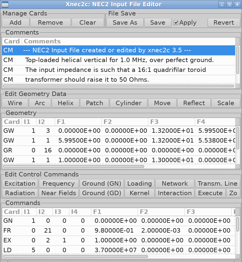
Xnec2c has a built-in NEC2 input file editor to make the edit/save/execute cycle easier and quicker. The main editor window opens from either the menu n or menu e items of the Main window. The menu item opens the editor with some default rows ("cards") that amount to a free space vertical dipole which serves as a simple example. The menu is used to edit a NEC2 input file that is already open in xnec2c.
The main NEC2 input file editor can be used to directly edit rows if desired and indeed this is the only method available for editing Comments. The editor though has several dedicated sub-editors for each of the type of card that is indicated in the Buttons above the Geometry and Commands Tree Views. The dedicated editor windows open when these buttons are clicked (to add a new row) or when a selected row is right-clicked by the user with the mouse.
Main Editor Description
The Main NEC2 Editor window is divided into three Tree View areas,
one for editing Comments, one for editing Geometry and one for
Control Commands. Each tree view has editable rows divided into
cells that correspond to NEC2 input file's card columns e.g. Card
Name (CM) - Comment Text or Card Name (GW) - Wire Data (I1 I2 F1 F2
F3 F4 F5 F6 F7) etc. The text of the first
CM card is displayed in the title bar of
the Main and Radiation Pattern windows, providing a quick
identification of the loaded model. Each row can be edited by selecting it with a
mouse click and then clicking on a cell. This requires detailed
knowledge of the format of each of the NEC2 input file "cards" and
so this method is only useful for editing comments.
The main editor is controlled by the top row of buttons: The
(Ctrl+a) button inserts a new blank row in whatever tree
view has been selected by a mouse click. The (Ctrl+r)
button deletes a row that was selected by a mouse click and the
(c) button deletes all rows in a selected tree view
and clears it. The (Ctrl+Shift+s) button opens a file
selector dialog for saving the data in the Editor to a NEC2 input
file. The (Ctrl+s) button writes data in the Editor to
an already open input file. The check button, when checked,
signals xnec2c to reload the edited input file for execution.
The Geometry and Commands tree views each have an
button that creates a
symbolic variable
SY card for the selected row's numeric
fields, converting literal values into named parameters.
SY expressions can also be typed directly into the numeric fields
of any card editor — for example, entering
L0/2 in the Y2 field of a GW wire editor substitutes
the half-length at evaluation time.
Note: In xnec2c versions earlier than v2.0-beta, due to the complex file opening process followed by NEC2 (many data sanity checks and initializations etc), reloading the input file resulted in all open windows (radiation pattern, frequency plots) to be closed. This was always an awkward situation and slowed down work in the NEC2 input file editor. As of xnec2c v2.0-beta, the user interface as well as a fair amount of code in xnec2c, have been modified so that as far as possible, when an edited NEC2 file is saved and reloaded, or another NEC2 file is opened, xnec2c will not close open Radiation Pattern or Frequency Plot windows and will not completely reset internally. This allows the user to edit a NEC2 file in the Editor window and, after saving, to be presented with the new calculations on the structure being modeled.
Finally the (Ctrl+r) button reloads the last saved state of the editor from the input file, to reduce the effort needed to recover from a big mistake like clearing a tree view accidentally!
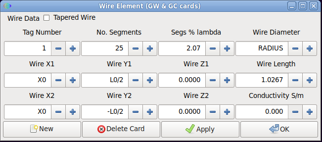
Sample Dedicated Geometry Editor Description
Wire Geometry Editor
This is one of the dedicated "card" or row editors, for creating or editing wire geometry. It will appear when the "Wire" button in the "Edit Geometry Data" frame is clicked or when a selected Wire row is right-clicked with the mouse. In the former case, a blankGW row will be added to the Geometry tree
view which can then be filled by entering wire geometry data in the
Editor and clicking Apply or OK. (in the latter case the editor is
closed). The "Tapered Wire" check button in the upper left corner
opens an additional frame for entering wire taper data and adds a
blank GC row to the tree view.
To make things easier, the Wire editor has spin buttons to specify Length Taper and Diameter Taper separately to hide the need for calculating the actual beginning and end diameters. Also the "Segs % λ" spin button indicates the wire segment length as a percentage of smallest λ and can be use to set the needed number of segments for each wire to maintain a uniform relative segment length for all wires.
Three geometry Editors (wire, helix, arc) have a spin button to
specify wire conductivity in S/m. When the spin button
value is greater than zero, the Editor will enter an LD card in the
Commands tree view to specify a type 5 (wire conductivity) loading.
This will result in all segments with tag number equal to that in
the Editor to be loaded with the specified resistivity.
All editors (except for the GE card) have the following
buttons along the bottom of the window: "New" inserts a new blank
row in the tree view after entering edited data into the current
row. "Delete Card" removes the current row (card) and closes the
editor window. "Apply" enters edited data into the current row.
"OK" enters edited data into the current row and closes the editor
window.
As of v3.9-beta, the GH "card" editor has a new
appearance, since the Helix producing code has been edited to allow
the creation of a spiral. Both right-hand/left-hand helices or
spirals can be specified with the radio buttons in the top row of
the GH editor dialog. In the bottom row, the radii that specify the
shape of helices or spirals can be entered in the relevant spin
buttons. These can be linked so that values entered can be
propagated to the right, to make editing easier if all radii are
the same. Right propagation is controlled by clicking on the "chain
link" icons - if the icon displays a linked chain, right
propagation is enabled. Otherwise if a broken link, right
propagation is disabled.
Sample Dedicated Control Editor
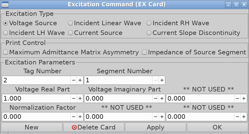
Excitation Command Editor
The Excitation Command Editor opens when the "Excitation" button in the "Edit Control Commands" frame is clicked or when a selectedEX row is
right-clicked with the mouse. The excitation type is selected by
activating the appropriate radio button whereby some labels over
the data input spin buttons will change to indicate their purpose.
The print control check buttons specify additional data to be
printed to the output file but please remember that xnec2c does not
produce an output file. The buttons in the bottom row of the
Command Editors function in the same way as the Wire editor
described above.
Symbolic Variables (SY) and Live Parameter Tuning
Antenna design often begins with a target frequency and a set of proportions—element lengths
expressed as fractions of wavelength, spacing ratios derived from empirical data or simulation
refinement. The SY card transforms these relationships from scattered
numeric literals into a coherent symbolic framework where changing one value ripples through
the entire model. This 4nec2-compatible extension brings parametric modeling to xnec2c,
enabling rapid exploration of design variations without manually editing dozens of coordinate
values.
SY Card Syntax
Symbol definitions appear in either the geometry or command section of the input file.
Each SY card declares one or more variables using the format:
SY name=value
SY name=expression
SY a=1, b=a*2, c=b+1
Comma separation allows multiple definitions on a single line, evaluated left-to-right
so that later symbols can reference earlier ones. Symbol names are case-insensitive;
FREQ, Freq, and freq all resolve to the same value.
Expressions support standard arithmetic operators (+, -,
*, /, ^) with conventional precedence.
Mathematical functions include trigonometric operations (SIN, COS,
TAN, ATN—note that angles are in degrees), square root
(SQR), exponential and logarithmic functions (EXP, LOG,
LOG10), and utility functions (ABS, SGN, INT,
FIX, MOD, MAX, MIN).
Predefined constants eliminate magic numbers from antenna descriptions:
The included example examples/2m_yagi_SY_parametric.nec demonstrates how symbols cascade through a model:
SY FREQ=146, C=299.792458, LAMBDA=C/FREQ
SY L_REF=0.492*LAMBDA, L_DRV=0.468*LAMBDA
SY X_DRV=0.193*LAMBDA, RADIUS=AWG_10
GW 1 25 0 L_REF/2 0 0 -L_REF/2 0 RADIUS
GW 2 25 X_DRV L_DRV/2 0 X_DRV -L_DRV/2 0 RADIUS
FR 0 21 0 0 FREQ-5 0.5
Changing FREQ recalculates wavelength, which propagates to element lengths
and positions—the entire antenna scales to a new band through a single edit.
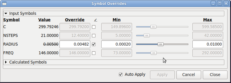
Symbol Overrides Window
Select to open the tuning interface.
The window displays all defined symbols in two collapsible sections: Input Symbols
contain direct assignments from SY cards, while
Calculated Symbols derive their values from expressions referencing other symbols.
Each row presents:
- Symbol name and its current evaluated value
- Override entry with checkbox—when enabled, this value supersedes the original definition during simulation
- Min/Max bounds defining the slider range
- Slider for continuous adjustment within bounds
- Expression (for calculated symbols) showing the source formula
When an override activates, the original value displays with strikethrough styling, providing visual confirmation that the symbol now draws from the override rather than its definition. Bounds auto-expand if slider movement or direct entry exceeds current limits—drag the slider past the maximum and the ceiling rises to accommodate the new value.
Auto-Apply Parameter Tuning
The Auto Apply checkbox transforms the Symbol Overrides window into a real-time tuning console. With this mode active, each slider adjustment or value change triggers an automatic sequence: a 300-millisecond pause allows rapid successive adjustments to coalesce, then xnec2c saves the override state, reloads the model, and recalculates all frequency points. A spinner indicates when calculations are in progress; additional changes queue until the current computation completes.
This mechanism integrates seamlessly with the optimization workflow. External scripts can modify the companion .sy file directly—xnec2c monitors both .nec and .sy files for changes, reloading automatically when either updates. The override file format stores symbol state in a straightforward text structure:
# Symbol overrides file
FREQ: min_value=100 max_value=200 override_value=146 override_active=1
LAMBDA: min_value=1.0 max_value=4.0 override_value=2.05 override_active=0
Override persistence means tuning sessions survive application restarts. The
.sy file loads before SY card
processing begins, pre-populating bounds and override values so that subsequent symbol
definitions merge with existing tuning state rather than replacing it. The
opt_active field marks whether each variable is included in built-in
optimizer runs.
Expressions in Card Editors
When SY symbols are defined, their expressions appear directly in geometry and command
card fields. Right-click a card row (such as a GW wire definition) in the NEC2 editor
treeview and select Edit, or double-click the row. The card editor dialog
shows coordinate fields populated with expressions — X1,
L1/2, -L1/2 — rather than raw numeric values. The editor
preserves these expressions through the edit cycle: changing a value and clicking OK
writes the expression back to the model.
Expression errors during editing are batched and shown in a single consolidated dialog rather than one popup per field.
Antenna Geometry Optimization
Xnec2c includes a built-in optimizer that adjusts SY symbolic variable values to improve antenna performance across the frequency sweep. The optimizer evaluates each candidate geometry by running a full NEC2 frequency sweep, computing a weighted fitness score from user-defined goals, and converging toward designs that minimize that score. This works directly with the Symbol Overrides window — variables marked for optimization are the search dimensions, and the override min/max bounds define the search space.
Three windows provide live feedback during optimization. Open all three before starting:
- — watch VSWR and gain evolve across the band as the optimizer tests candidates
- — observe beam shape changes in real time
- The main Structure window — see geometry adjust as variables change
While the optimizer is running it controls the frequency sweep exclusively. The frequency spin buttons in both the Main and Radiation Pattern windows are disabled, and frequency plot traces turn dark green to indicate that the sweep is managed by the optimizer. Clicking in the plot area to select a frequency is also blocked during this time. All controls are restored when the optimizer finishes or is stopped.
For the historical external-optimizer approach (where a separate program modifies the .nec file while xnec2c monitors for changes), see External Optimizers below.
Quick Start: Optimizing an Example Antenna
This walkthrough uses examples/5el_yagi_SY_parametric.nec, which ships with a pre-configured .opt file containing fitness goals for VSWR, gain, and beam direction. The companion .sy file is created automatically the first time you interact with Symbol Overrides.
Understanding the Parametric Model
The antenna's shape emerges from a chain of symbolic relationships. Each variable controls one aspect of the physical structure:
R0,R1,R2,R3— element length ratios- Each director derives its length from the preceding element multiplied by its R factor:
L1=L0*R0,L2=L1*R1, and so on. Values of R below 1.0 enforce the forward tapering required of a Yagi — each director shorter than the one behind it. Without this constraint the optimizer could produce geometries where a forward director grows longer than the reflector, violating the fundamental operating principle of a Yagi-Uda array. The expressions that define the geometry must represent the intended physical outcome, because the optimizer will find and exploit any freedom the model leaves unconstrained. S0,S1,S2,S3— element spacing (wavelength fractions)- Spacing between adjacent elements as fractions of wavelength, accumulated from the
preceding element:
X1=X0+S0*LAMBDA,X2=X1+S1*LAMBDA, etc. Absolute positions would allow the optimizer to place a director behind the reflector or reverse the element order entirely — geometries that have no meaning as Yagi designs. Cumulative offsets prevent this while directly controlling the coupling between adjacent elements, which determines impedance matching, bandwidth, and gain distribution across the sweep. X0— reflector position- Fixed at 0, serving as the coordinate origin. Moving the entire antenna through space changes nothing about its electrical properties, so this variable is not checked for optimization.
L_REF_SCALE— reflector half-length scale factor- Scales the reflector:
L0=0.5*LAMBDA*L_REF_SCALE. Because L0 is the root of the multiplicative length chain — every director length ultimately derives from it through successive R factors — adjusting this single value rescales the entire antenna proportionally. Left at 1.0 in this example, though it can be optimized when the reflector length needs independent adjustment relative to the wavelength-scaled default. RADIUS— wire radius- Unchecked in this example. Wire radius affects impedance and bandwidth but is
typically determined by available tubing stock rather than optimization. For designs
where wire diameter is a significant fraction of segment length, see the
EKcard.
Tutorial Steps
- Open examples/5el_yagi_SY_parametric.nec.
- Enable the frequency sweep and open plot windows: select , enable VSWR and Max Gain graphs, and click the triangular Play button. Also open .
- Note the baseline performance: maximum gain is approximately 10.57 dBi, but worst-case VSWR across the band reaches 5.68. Even at the peak gain frequency, VSWR is nearly 3.0 — far above the 2.0 threshold where most transmitters begin folding back power.
- Open .
- Check the Opt checkbox for
R0,R1,R2,R3,S0,S1,S2,S3— these are the design variables the optimizer will adjust. - In the Optimization expander, the .opt file has pre-configured fitness goals: minimize VSWR (target 1, weight 5), maximize Max Gain (target 12, weight 10), and minimize Gain Dev +X (target 1, weight 10). The third goal constrains the direction of maximum gain to lie along the +X boom axis. Without it, the optimizer could produce geometries where gain is high but the beam points off-axis — a parasitic array resembling a dipole with reflector wires on either side, or a design that radiates strongly in elevation rather than toward the horizon. Directional constraint ensures the optimizer pursues high gain only in the intended forward direction.
- Select Particle Swarm (PSO) and click Start
Optimization. Watch all three windows update as the swarm explores the design
space. The status bar reports progress:
Pass N/M Iter Evals Fitness Best Stagnant Cache. - When PSO completes, switch to Simplex and click Start Optimization again. Simplex refines the best solution PSO discovered, descending precisely into the nearest minimum — a complementary strategy to the broad search that preceded it.
- After Simplex completes: worst-case VSWR has dropped to approximately 1.19, with most of the band below 1.07, and maximum gain measures about 10.14 dBi. The peak gain decreased slightly from the unoptimized value because the optimizer found a geometry that distributes performance evenly across the band rather than concentrating it at a single frequency. The antenna is now usable from end to end. Optimization is stochastic — both PSO and Simplex involve random initial conditions — so exact results will vary between runs, but should fall in the same general range.


Iterative Refinement
The weight and exponent values for each fitness goal determine how the optimizer balances competing objectives. Increasing VSWR weight prioritizes impedance match quality at the expense of gain; increasing gain weight does the reverse. Higher exponents penalize large deviations more severely than small ones — an exponent of 2 squares the penalty, making a measurement twice as far from target four times as costly.
When an optimization run produces unexpected results — gain that seems too low, or VSWR that the optimizer ignores in favor of another metric — the Score column in the fitness goals grid reveals where the optimizer is spending its effort. A goal with a large score relative to the others dominates the total fitness and steers the search; goals with small scores have little influence regardless of how far their measurements sit from target. To shift the balance, increase the weight or exponent of an under-represented goal so its penalty grows large enough to compete, or reduce those values on an over-represented goal to loosen its grip on the search. The formula display at the bottom of the grid confirms the effect: re-run a pass after adjusting and compare the per-goal score breakdown to verify that the optimizer now distributes attention across all objectives as intended.
Subsequent passes of the same algorithm start from the current best values and often discover nearby improvements the first pass missed. When switching between algorithms, the key parameter to adjust is the search region: reduce PSO's Search size on later passes to concentrate the swarm near the current solution instead of scattering particles across the full range. For Simplex, the Sizes list already defines a sequence of decreasing perturbations — each pass automatically uses the next smaller entry.
Performance note: optimization runs faster when near-field calculations are disabled. Uncheck NH/NE output in the command cards or disable current display in the structure window. Near-field computation adds overhead to every frequency step and is unnecessary when only gain pattern and VSWR matter.
Fitness Goals and Measurement Types
Each optimization objective occupies one row in the fitness goals grid, defining what the optimizer should improve and how aggressively it should pursue that improvement. The total fitness score — the single number the optimizer minimizes — is the weighted sum of all enabled goals evaluated across the frequency sweep.
Use the + Add Metric button to append a new goal row, or the −
button on any existing row to remove it. The formula display at the bottom shows the
complete fitness calculation:
F = W1*reduce((transform)^exp) + W2*... = total.
Goal Row Columns
- Enable (checkbox)
- Include or exclude this goal from the fitness calculation. Disabled goals remain configured but contribute nothing to the score.
- Measurement (combo box)
- The antenna parameter to evaluate. See the measurement reference table below.
- Value (read-only)
- The current measured result, updated live during optimization from the best candidate's frequency sweep.
- Transform (direction combo box)
- How the raw measurement converts to a penalty score:
- min score —
score = (max(v − t, 0) / √(t² + 1))exp + τ / (1 + max(t − v, 0) / √(t² + 1)). Penalizes values above target; score approaches zero as value improves below target. A small tension term τ provides a residual gradient so the optimizer continues to improve met objectives. Appropriate for VSWR, angular deviation, S11 return loss, and any metric where smaller readings indicate better performance. - max score —
score = (max(t − v, 0) / √(t² + 1))exp + τ / (1 + max(v − t, 0) / √(t² + 1)). Penalizes values below target; score approaches zero as value improves above target. Works correctly for both positive and negative targets. Appropriate for gain, front-to-back ratio, G/T, and metrics where larger readings indicate improvement. - ± target —
score = |value − target|exp. Penalizes deviation from target; score is zero when value equals target. Appropriate for impedance, phase angle, beam pointing, and metrics that converge on a specific number rather than an extreme.
- min score —
- Target
- The goal value for the selected measurement. Its meaning depends on the transform direction: for min score, the upper threshold (score approaches zero below this value); for max score, the lower threshold (score approaches zero above this value); for ± target, the center point of zero penalty. The √(t² + 1) normalization smoothly transitions between relative error for large targets and absolute error near target zero, with the crossover at |target| = 1.
- Exp (exponent)
- Applied to the transform result before reduction. Controls penalty steepness: an exponent of 1 produces linear scaling, 2 produces quadratic growth that penalizes large deviations disproportionately, and 0.5 compresses the range so that large and small deviations contribute more equally.
- Reduce (reduction combo box)
- How scores from individual frequency steps combine into a single value for this goal:
- sum — adds every frequency step's score; total grows with the number of steps, weighting broadband compliance heavily
- avg — averages across steps; normalizes for step count, balancing contribution across the band
- min — selects the lowest-penalty step. This isolates the single frequency where performance is strongest, which suits single-frequency or narrow-band designs where only the best operating point matters and the rest of the sweep serves as context rather than constraint
- max — selects the highest-penalty step, forcing the optimizer to improve the worst point in the band; effective for ensuring minimum performance everywhere
- mag — root of summed squared scores:
sqrt(Σ score²); emphasizes large outliers without ignoring small ones - diff — spread between largest and smallest scores; penalizes uneven performance across the band, pushing toward flat response
- Weight
- Multiplier applied after reduction. Determines relative importance when multiple goals compete — a goal with weight 10 has twice the influence of one with weight 5.
- MHz lo / MHz hi
- Optional frequency band filter. When set, only frequency steps within this range contribute to the goal's score. Empty values include all frequencies from the FR card. Filtering allows different objectives for different portions of the band — for example, strict VSWR within a 500 kHz operating segment while allowing relaxed gain tolerance across the full sweep.
- Score (read-only)
- Current penalty score for this objective, updated live.
Measurement Reference
| Measurement | Description | Default Direction | Default Target |
|---|---|---|---|
| Z Real | Real part of feed-point impedance (Ω) | ± target | 50.0 |
| Z Imaginary | Imaginary part of feed-point impedance (Ω) | ± target | 0.0 |
| Z Magnitude | Magnitude of feed-point impedance (Ω) | ± target | 50.0 |
| Z Phase | Phase angle of feed-point impedance (°) | ± target | 0.0 |
| VSWR | Voltage standing wave ratio (1.0 = perfect match) | min score | 1.0 |
| S11 | Return loss in dB (more negative = better match) | min score | −15.0 |
| S11 Real | Real part of S11 in dB | min score | −15.0 |
| S11 Imaginary | Imaginary part of S11 in dB | ± target | 0.0 |
| S11 Angle | Phase angle of reflection coefficient (°) | ± target | 0.0 |
| Max Gain | Peak gain across all angles (dBi) | max score | 12.0 |
| Net Gain | Peak gain adjusted for mismatch loss (dBi) | max score | 6.0 |
| Gain Theta | Elevation angle of peak gain (°) | ± target | 90.0 |
| Gain Phi | Azimuth angle of peak gain (°) | ± target | 0.0 |
| Viewer Gain | Gain toward current viewer angle (dBi) | max score | 6.0 |
| Viewer Net Gain | Viewer gain adjusted for mismatch loss (dBi) | max score | 6.0 |
| F/B Ratio | Front-to-back ratio (dB) | max score | 20.0 |
| Gain Dev +X | Angular deviation of peak gain from +X axis (°) | min score | 1.0 |
| Gain Dev −X | Angular deviation of peak gain from −X axis (°) | min score | 1.0 |
| Gain Dev +Y | Angular deviation of peak gain from +Y axis (°) | min score | 1.0 |
| Gain Dev −Y | Angular deviation of peak gain from −Y axis (°) | min score | 1.0 |
| Gain Dev +Z | Angular deviation of peak gain from +Z (zenith) (°) | min score | 1.0 |
| Gain Dev −Z | Angular deviation of peak gain from −Z (nadir) (°) | min score | 1.0 |
| T_ant | Antenna noise temperature T_ant from sky/earth brightness (K) | min score | 1000.0 |
| T_total | Total system noise temperature T_total including ohmic loss (K) | min score | 1000.0 |
| G/T_ant | Gain-to-antenna-temperature ratio (dB), excludes loss | max score | 5.0 |
Noise Optimization Workflow
Tant, Ttotal, and G/Tant depend on the observation elevation set in the T Elev° control and the selected noise environment. Set both to their intended operating values before starting an optimization pass that includes noise objectives.
A two-stage approach produces the best results. In the first pass, optimize for antenna geometry and pattern behavior—gain, VSWR, F/B ratio, beam direction—without noise objectives. This establishes a sound electrical design. In subsequent passes, add Tant or G/Tant objectives to refine noise performance at the intended elevation. Combining both stages in a single pass risks the optimizer distorting the pattern geometry to chase a noise figure that depends on an elevation angle it cannot control.
Algorithm Selection and Advanced Settings
The algorithm selector in the Optimization expander offers two choices. A ? button beside the selector opens context-sensitive help describing the currently selected algorithm's parameters.
Common Settings
- Stagnation count (default: 30)
- Iterations without improvement before the current pass ends.
- Tolerance (default: 0.001)
- Minimum improvement threshold — changes smaller than this are not counted as progress toward the stagnation limit.
- Max iterations (default: 100)
- Hard cap per pass regardless of improvement rate.
Simplex (Nelder-Mead)
The Simplex algorithm constructs a geometric shape (simplex) in the space of optimization variables and iteratively moves its vertices toward lower-fitness regions through reflection, expansion, and contraction operations. It excels at refining a solution that is already near a good region.
- Sizes
- Comma-separated initial simplex sizes for multi-pass operation (e.g.,
0.09, 0.075, 0.05, 0.025). Each pass uses the next entry, producing progressively finer refinement. The number of entries determines the number of passes. - Min size (default: 1e-06)
- Convergence threshold for simplex diameter. When the simplex contracts below this size, the pass ends — the algorithm has exhausted the region it can usefully explore.
- Temperature (default: 0)
- Simulated annealing temperature. At 0, the algorithm runs as pure Nelder-Mead, accepting only improvements. Positive values introduce random uphill moves proportional to the temperature, intended to escape shallow local minima. In practice this is difficult to tune effectively — PSO with an appropriate search size is generally a more reliable approach to escaping local minima, since the swarm naturally covers a wider region without requiring temperature calibration.
PSO (Particle Swarm Optimization)
PSO distributes a swarm of candidate solutions across the search space. Each particle tracks its own best-found position and is attracted toward both that personal best and the best position found by its neighborhood. The balance between exploration (inertia) and convergence (cognitive and social attraction) determines how quickly the swarm collapses toward a solution.
- Particles (default: 0 = auto)
- Swarm size. When set to 0, the count is calculated automatically from the number of optimization variables. Larger swarms explore more thoroughly at the cost of more function evaluations per iteration.
- Neighbors (default: 0 = auto)
- Neighborhood size for the social component. Each particle is influenced by the best position within its neighborhood rather than the global best, which preserves diversity and reduces premature convergence.
- Inertia (default: 0.9)
- Velocity decay factor. Values near 1.0 maintain momentum and favor exploration; lower values increase damping and favor convergence.
- Cognitive (default: 0.5)
- Attraction strength toward each particle's personal best position.
- Social (default: 0.5)
- Attraction strength toward the neighborhood best position.
- Search size (default: 0.25)
- Initial random spread for particle positions, expressed as a fraction of each variable's min-max range and applied as a ± offset from the starting point. A value of 0.25 places particles within 50% of the total range centered on the current values. If the resulting positions exceed a variable's bounds, they are clamped to the boundary. On subsequent passes, reducing this value concentrates the swarm near the current best solution rather than scattering across the full range.
Status Bar
During optimization the status bar displays:
Pass 4/4 Iter 47 Evals 330 Fitness 19.9103 Best 19.9103 Stagnant 46 Cache 0/330 [Complete]
Optimizer Configuration Files (.opt)
The optimizer stores its configuration in a .opt file alongside the .nec file, using GKeyFile INI format. The file is auto-saved on every widget change and auto-loaded when opening a .nec file if a matching .opt file exists. See examples/5el_yagi_SY_parametric.opt for an annotated example of the format.
External Optimizers
As an alternative to the built-in optimizer, external programs can optimize antenna geometry through a file-monitoring feedback loop. Neoklis, 5B4AZ first described this approach:
Xnec2c monitors its .nec input file for changes and re-runs the frequency stepping loop which recalculates new data and prints to the .csv file. It is therefore possible to arrange the optimizer program to read the .csv data file, recalculate antenna parameters and save them to the .nec input file. xnec2c will then recalculate and save new frequency-dependent data to the .csv file.
If the optimizer program is arranged to monitor changes to the .csv file, then a continuous loop can be created in which new antenna parameters are calculated and saved to the .nec file, new frequency dependent data are calculated and saved to the .csv file and the loop repeated until the desired results (optimization) are obtained.
This mechanism was first implemented in Xnec2c v4.2. External optimizers remain useful for custom fitness functions, genetic algorithms, or specialized workflows not covered by the built-in optimizer. The following packages are available:
- Xnec2c-gao is an external optimizer that uses a genetic algorithm to find solutions in a multidimensional search space. It is written in Haskell by Maurizio Di Pietro and hosted on github.
- Xnec2c-optimize is written in Perl by Eric Wheeler and hosted on github.
Activating .NEC File Monitoring
Xnec2c will monitor the currently open .NEC file when you select
and select "Reload and write data on .NEC file
changes". Additionally, you need to tell xnec2c where to write its output
file. You can do that with one of the --write-* command-line options
or by checking one of the boxes in such as
"After calculation, write <file>.csv".
The checkbox
"After calculation, write <file>-structure.gplot"
exports a gnuplot-compatible 3D structure file after each evaluation.
The checkbox
"After calculation, write <file>-patch-currents.csv"
exports surface patch current data in CSV format.
All output settings are persisted in the configuration file.
Enable the frequency sweep if it is not already turned on:
- From the main window: select
- From the Frequency Data Plots window: enable a graph such as VSWR, and configure whatever you would like to see during optimization.
- Click the triangular "Play" button to run a frequency sweep. This is a persistent setting that will auto-sweep each time xnec2c loads and it must be active in order for the optimizer loop to function.
Frequency loop timing information is available on the console when you increase
verbosity with -v. Specify -v multiple times to increase
verbosity. For example, with -vv using examples/2m_yagi.nec:
[info] 140.000000 MHz: 0.045850 seconds. (ATLAS, Threaded)
[info] 141.500000 MHz: 0.054378 seconds. (ATLAS, Threaded)
[info] 140.000000 MHz: 0.063772 seconds. (ATLAS, Threaded)
[info] 140.500000 MHz: 0.066472 seconds. (ATLAS, Threaded)
[info] 141.000000 MHz: 0.078861 seconds. (ATLAS, Threaded)
[info] 142.000000 MHz: 0.047910 seconds. (ATLAS, Threaded)
[info] 143.000000 MHz: 0.068066 seconds. (ATLAS, Threaded)
[info] 143.500000 MHz: 0.076449 seconds. (ATLAS, Threaded)
[info] 144.000000 MHz: 0.068083 seconds. (ATLAS, Threaded)
[info] 142.500000 MHz: 0.113185 seconds. (ATLAS, Threaded)
[info] 146.000000 MHz: 0.050178 seconds. (ATLAS, Threaded)
[info] 144.500000 MHz: 0.051486 seconds. (ATLAS, Threaded)
[info] 145.000000 MHz: 0.058897 seconds. (ATLAS, Threaded)
[info] 145.500000 MHz: 0.060019 seconds. (ATLAS, Threaded)
[info] 147.000000 MHz: 0.057313 seconds. (ATLAS, Threaded)
[info] 146.500000 MHz: 0.070968 seconds. (ATLAS, Threaded)
[info] 148.000000 MHz: 0.071760 seconds. (ATLAS, Threaded)
[info] 147.500000 MHz: 0.080575 seconds. (ATLAS, Threaded)
[info] 148.500000 MHz: 0.051870 seconds. (ATLAS, Threaded)
[info] 149.500000 MHz: 0.058890 seconds. (ATLAS, Threaded)
[info] 150.000000 MHz: 0.056449 seconds. (ATLAS, Threaded)
[info] 149.000000 MHz: 0.071011 seconds. (ATLAS, Threaded)
[notice] Frequency loop elapsed time: 0.467847 seconds. (ATLAS, Threaded)
Input File Considerations
Since xnec2c is interactive, it will not initiate calculations
without a prompt from the user. For this reason certain NEC2
commands that normally cause execution (e.g. RP, XQ etc) are read
in but not acted upon. Any data in the lines of these commands are
saved for use when the user requests output data calculation and
display, via buttons and menu items in the GUI. Also, since xnec2c
was designed to visualize output data graphically, certain types of
output data requests are not supported (e.g. the surface wave
pattern option (I1 = 1) of the RP command etc). An error message
dialog will hopefully appear to inform the user of unsupported
commands or options.
Since xnec2c is an implementation of NEC2. You can learn more about the NEC2 format at https://www.nec2.org. Be sure to review Part III: NEC User's Guide. Here is a list of commands or command options not supported by xnec2c:
GF- Read Numerical Green's Function: Relevant code has been removed in nec2c since this type of solution is obsolete.
WG- Write Numerical Green's Function: Relevant code has been removed in nec2c since this type of solution is obsolete.
NX- Next Structure Data: Relevant code has been removed since xnec2c cannot operate in batch mode.
PQ,PT,CP- These commands affect printed output and have no effect on data presented by xnec2c in graphical form. Since v1.0 xnec2c does not print results to file.
SOMNEC- The separate SOMNEC code has been incorporated in nec2c and hence in xnec2c also.
EK- Activates the extended thin-wire kernel. The standard kernel treats each wire segment as an infinitely thin current filament — current flows along a line at the wire axis and the boundary condition is enforced approximately at the surface. The extended kernel incorporates the wire's finite radius into the field evaluation, accounting for the cylindrical geometry when computing interactions between nearby segments. This produces more accurate results when the segment length-to-radius ratio is small: the standard kernel requires a ratio of at least 8 for 1% field accuracy (minimum usable: 2), while the extended kernel achieves 1% accuracy at a ratio of 2 (minimum usable: 0.5). The additional computation per segment is negligible on modern hardware, so enabling EK is generally recommended. Xnec2c reports accuracy warnings when geometry violates the active kernel's validity conditions.
EX- When Incident Wave or Elementary Current Source Excitation is specified, xnec2c can only calculate and render the re-radiated field, produced by the current induced onto the structure. Only the initial values of the θ and φ angles are used and no stepping of these angles is performed. Therefore it is better to specify only one step for θ and φ in the
EXcard. RP- The surface wave option (I1 = 1) is not supported.
SY- Symbolic variable definition for parametric modeling, compatible with 4nec2. Defines named constants and expressions that substitute into geometry and command card fields. See SY Symbolic Variables and Parameter Tuning for full documentation.
Z0- Specifies the transmission-line reference impedance Z0 in the NEC2 antenna description file. The mnemonic is canonically
Z0(digit zero); legacy decks written withZO(letter O) still parse.
Output File Considerations
Printing of results to an output file has been removed starting from v1.0, since xnec2c works in a way that does not allow printing compatible with the NEC2 format. If printing to file is needed then it is better to use the original NEC2 program, to avoid bugs that may still be lurking in the C translation.
Keyboard Shortcuts
The following tables summarize all keyboard accelerators. Single-key shortcuts are active when the corresponding window has focus. Modifier combinations work regardless of widget focus within the window.
Main Window
| Key | Action |
|---|---|
| n | File → New |
| o | File → Open |
| e | File → Edit NEC2 input |
| s | File → Save |
| Ctrl+s | File → Save As |
| Ctrl+q | Quit |
| r | Open Radiation Pattern window |
| f | Open Frequency Data window |
| i | Toggle Currents display |
| v | Toggle Charges display |
| x | X axis view preset |
| y | Y axis view preset |
| z | Z axis view preset |
| d | Default view preset |
| Ctrl+Plus | Zoom in |
| Ctrl+Minus | Zoom out |
| Ctrl+1 | Zoom 100% |
| Ctrl+Scroll | Adjust wire cylinder scale (OpenGL) |
Radiation Pattern Window
| Key | Action |
|---|---|
| n | File → New |
| o | File → Open |
| e | File → Edit NEC2 input |
| s | File → Save |
| Ctrl+s | File → Save As |
| Ctrl+q | Quit |
| g | Toggle Gain pattern display |
| f | Toggle E/H Near Field display |
| X | X axis view preset |
| Y | Y axis view preset |
| Z | Z axis view preset |
| d | Default view preset |
| a | Apply frequency / recalculate |
| Ctrl+Plus | Zoom in |
| Ctrl+Minus | Zoom out |
| Ctrl+1 | Zoom 100% |
| Ctrl+Scroll | Adjust wire cylinder scale (OpenGL) |
| Shift+Scroll | Scale structure overlay (OpenGL, gain view only) |
Frequency Data Window
| Key | Action |
|---|---|
| n | File → New |
| o | File → Open |
| e | File → Edit NEC2 input |
| s | File → Save |
| Ctrl+s | File → Save As |
| Ctrl+q | Quit |
| m | Toggle Max Gain plot |
| d | Toggle Directivity plot |
| w | Toggle Net Gain plot |
| v | Toggle VSWR plot |
| z | Toggle Impedance plot |
| p | Toggle S11 plot |
| l | Linear frequency scale |
| h | Logarithmic frequency scale |
| b | Both (linear + log) frequency scale |
NEC2 Editor
| Key | Action |
|---|---|
| Ctrl+a | Add row |
| Ctrl+r | Remove row / Revert |
| Ctrl+s | Save |
| Ctrl+Shift+s | Save As |
| c | Clear selected tree view |
Version History (newest first)
Version 5.0
This release adds hardware-accelerated OpenGL rendering, an integrated antenna geometry optimizer with three algorithms, symbolic variable parametric modeling, noise temperature analysis, current flow visualization, and internationalization support.
- Contributors:
- frazij — suggested displaying model filename in window titles (#77)
- G1OGY — reported WSL2/Debian compile failure (#78)
- malcolmboyd — reported optimizer single-frequency issue (#62)
- Peter3579 — tested and validated the Touchstone format for antenna gain in the virtual two-port model (#80), and reported the frequency-plot readout defect (#82)
- Ian — reproduced and tested the
Z0-card value corruption (#86) - peteasa — drove the
--write-patch-currentsoption and the gnuplot patch-line fix (#75, #76) - 9M2PJU — reported a build break and submitted a pull request (#84, #85)
- OpenGL rendering (documentation):
- Hardware-accelerated 3D renderer with lit cylinder geometry, triangulated patch surfaces, smooth vertex normals, coordinate axes with labels, and ground plane visualization
- OpenGL Settings dialog: per-element brightness and transparency sliders, MSAA anti-aliasing (Off/2×/4×/8×/16×), cylinder scale, and draw style selection
- Orthographic projection toggle in both Main and Radiation Pattern window toolbars (documentation)
- Radiation pattern draw style: Surface, Wireframe, or Both (documentation)
- Gradient key (color legend) visibility toggle
- Structure overlay in radiation pattern view with Shift+Scroll scaling
- Interactive wire cylinder radius via Ctrl+Scroll with line-mode snap at minimum
- Patch current visualization with five modes: Reference Phase, LIC Texture, Wireframe, Polarization Axis, and Peak Magnitude (documentation)
- Automatic Cairo software renderer fallback when OpenGL is unavailable
- Network and transmission-line
(
NT/TL) connections drawn in 3D, reaching parity with the Cairo renderer
- Color projection and tone mapping
(documentation):
- Current color projection axes: Dual current and charge, Standing and Traveling wave, and Far-field contribution
- Tone-transfer families for the color scale: dB, Asinh, mu-law, Reinhard, Sigmoid, and None
- Animate dialog rebuilt as a standalone panel with a manual phase-scrub slider (0–720°), mirror checkboxes, a flow-direction selector, and node/antinode and comet wire overlays
- Frequency-plot enhancements
(documentation):
- Six built-in color themes under with an Invert toggle and user override via ~/.xnec2c/themes.ini
- Detachable single-graph popups opened by double-clicking a graph or right-clicking a plot-select button, each carrying its own readout bar and closed with Ctrl+W
- Per-feedpoint excitation-port selector choosing which
EXfeedpoint drives the impedance, VSWR, and Smith data of a view - Feedpoint-dependent panels grey with explanatory tooltips and em-dash readouts when the excitation defines no feedpoint
- Interactive Smith chart with a full resistance and reactance grid, wavelengths-toward-generator scale, and click-to-select frequency
- Swap-click frequency selection, a persisted toggle that inverts the left and right mouse frequency-pick actions
- Symbolic variables and parametric modeling
(documentation):
SYcard support for named constants and expressions, compatible with 4nec2- SY expressions can be entered directly in NEC2 card editor
numeric fields (e.g.,
L0/2in a GW wire Y2 field) - Add Var (SY) buttons in NEC2 editor Geometry and Commands toolbars for converting literal values to named parameters
- Symbol Overrides window for interactive parameter tuning with min/max bounds, collapsible sections, and auto-apply
- External .sy override files for scripted parameter sweeps
- Antenna geometry optimization
(documentation):
- Built-in optimizer with Particle Swarm (PSO), Nelder-Mead Simplex, and Simple named-variable algorithms
- Dynamic fitness goals with selectable measurements, per-goal frequency band filtering, and threshold-based scoring
- Persistent .opt configuration files with auto-save
- Frequency controls locked during optimization with visual feedback (dark green plot traces)
- Gnuplot structure export and patch currents CSV output options
- inotify file watching for external optimizer compatibility
- Noise temperature and measurements
(documentation):
- Noise temperature visualization with eight environment models (VE7BQH, G4CQM, ITU-R) and adjustable observation elevation
- Antenna temperature (Tant), total noise temperature (Ttotal), and G/T figure of merit readouts in Frequency Plots and Radiation Pattern windows
- Average power gain diagnostic with efficiency percentage, auto-enabled with RP card (documentation)
- Radiation efficiency transmitted in frequency analysis for accurate G/T computation
- User interface:
- First
CMcard text displayed in Main and Radiation Pattern window title bars - Animation dialog reworked: Frames/Sec (1–120) replaces Steps/Cycle with auto-apply on value change
- Extended rotation range (0–720°) and incline range (±360°) with mouse-wheel scrolling on spin buttons
- Configuration file selection via
--configand--new-configCLI options --skip-verifyoption to improve load time on large models- Batch mode (
--batch) with--optimizefor headless optimization runs - All checkbox menu item states persisted in configuration file across sessions
- Transmission-line reference-impedance card is canonically
Z0(digit zero); legacyZOdecks still parse --write-validation-diroption to write the full validation data tree
- First
- Internationalization
(documentation):
- 42 languages via GNU gettext, selected automatically from system locale
LANGUAGEenvironment variable override
- Examples:
- ISS communication antenna designs (2m-5el-rhcp-ARISS-KJ7NLL.nec and 70cm-5el-rhcp-KJ7NLL.nec, 5-element RHCP Yagis by Zeke)
- Parametric Yagis with optimizer configuration (2m_yagi_SY_parametric.nec, 5el_yagi_SY_parametric.nec)
- Current-slope and current-source excitation demonstrations (ex2_current_slope_disc_dipole.nec, ex4_current_source_sq_loop.nec)
- Network transmission-line example (20m_dipole_NT_50ohm.nec)
- Bug fixes:
- Fix frequency loop re-entrancy and SY optimizer inotify reload races
- Fix fmhz_save clobbered by programmatic spinbutton updates
- Fix double unlock of global_lock mutex
- Fix single frequency step not running frequency loop (#62)
- Fix gradient legend invisible in Cairo renderer
- Fix compiler warnings on stricter build systems (#78)
- Replace GMutex with GRecMutex to prevent recursive lock deadlocks
- Fix sky/earth boundary calculation using Rodrigues rotation
- Fix inotify watch for atomic editor writes
- Fix stale geometry after SY variable apply
- Correct Sommerfeld ground accuracy (gshank L1-norm, evlua
contour completion) so feed-point impedance over
GN 2ground converges to the FORTRAN reference - Fix
Z0-card value corruption (#86)
- Build system:
- OpenGL and Epoxy are optional build dependencies
(
--enable-opengl) - Support running from source tree without installation
- OpenGL and Epoxy are optional build dependencies
(
Version 4.4.18
This release focuses on mathlib enhancements, platform compatibility improvements for MacOS and Fedora, and crash prevention through input validation.
- Contributors:
- Features:
- Thread count control via CLI options (
--openblas-threads,--mkl-threads,--omp-threads) - MacOS MacPorts OpenBLAS support
- Mathlib ID-based configuration for stable config persistence across version upgrades
- Thread count control via CLI options (
- Bug Fixes:
- Documentation:
- Thread control options documented in man page and HTML documentation
- Build system:
- Fix CFLAGS handling in spec file to preserve OpenMP flags
Version 4.4.17
This release includes radiation pattern color legend enhancements, critical bug fixes for locale handling and CSV output, stability improvements, and build system updates.
- Contributors:
- Ian - color legend suggestions, reported #61
- Neoklis Kyriazis - technical guidance on current scaling (#61)
- Devin Bayer - fixed double-free crash in geometry editor (#67)
- hamarituc - reported #59
- ProtonTheFox - reported #44, #45
- likecabezon - reported #68
- Jerry - reported #52
- polprog - reported #50
- roberthadow - reported #47
- Features:
- Graduated color legend with relative/absolute gain marks (-3dB, -6dB, -10dB intervals)
- Color legend with dynamic spacing and proper gain scaling
- Increased 3D zoom limit to 999999x
- GTK menu tear-offs for frequently used menus
- "Begin Frequency Loop at Startup" config checkbox (#45)
- Smooth pan/tilt/zoom during optimization
- Responsive mobile support for HTML documentation
- Bug Fixes:
- Fix NEC file format to use decimal points regardless of locale (#59)
- Fix CSV output scaling for currents/charges magnitude (#61)
- Fix double-free crash when editing geometry (#67)
- Prevent deadlocks in
Notice(),Open_Input_File(), and dialog scenarios - Fix endless loop with overlapping segments
- Fix gain value display and color mapping
- Improve error messages for segment tag lookup failures (#68, #47)
- Fix custom frequency step in color legend
- Fix radiation pattern color legend to match gain scaling styles
- Prevent GTK beeps (#50)
- Fix batch mode auto-start (#44)
- Graceful child process exit handling
- Reduce severity of math library detection failures to warnings
- Documentation:
- Build system:
- Add VSCode integration with debug configs and auto-configure
- Generate c_cpp_properties.json from configure
- Parallel build tasks support
Version 4.4.16
- Bug Fixes:
- Fixed geometry calculations when reading NEC2 decks that use the
GMcard withtag=0to copy all segments - Fixed segment lookup failures when
tag=0is specified - Improved error message to properly identify which
GMcard caused lookup failures - Improved radiation pattern color legend spacing
- Fixed building on sparc64
- Fixed geometry calculations when reading NEC2 decks that use the
- Code cleanups and improvements
- Contributors:
- Diane Bruce - inspired code cleanup and helped with pull requests
- Dave Hibberd - Debian maintainer who helped troubleshoot and provide guidance in solving the sparc64 build issue
Version 4.4.15
This release fixes a crash related to a GTK icon problem. Thanks to AsciiWolf for helping report and troubleshoot the issue.
Version 4.4.14
This release fixes a hang when the frequency plots window is too small for the number of plots being rendered. Thanks to Tom who reported the issue.
Version 4.4.13
This is a large bug-fix release and includes a few minor features and documentation updates. I would like to thank the following who helped with new features and bug fixes, in order of contribution:
- Contributors:
- Neoklis Kyriazis
- Rafal Lukawiecki
- ndim
- anoduck
- rklasen
- Ward
- ChrisMaple
- Features:
- Save window positions when they are closed
- Tile rdpattern and freqplot windows on first run
- Default the Radiation Pattern "Gain Pattern" to be enabled
- Officially support OpenBSD, thanks anoduck for testing
- Add save radiation pattern to CSV
- Add save currents and charges to CSV
- Documentation:
- Added External Optimizers section
- Added Google Translate javascript for the website
- Bug Fixes:
- Fixed deadlock when the frequency loop is running and a window is closed. Thanks to Neoklis Kyriazis for discovering the problem and proposing
a solution.
- Fixed edge case where structure window does not redraw on save. Thanks to Neoklis Kyriazis for discovering the problem and providing a fix.
- Fix blank plots, structures and radiation pattern when Quit is pressed.
- Open the Frequency Plots window when Optimization is enabled
- Auto-run freq loop when optimization is enabled
- Differentiate between windows at 0,0 and never opened
- Correct a relatively trivial warning from Coverity Scan about an unused value
- Fix warning from Coverity Scan about invalid argument to a function
- Fix a warning by Coverity Scan about an unterminated buffer
- Fix Coverity Scan warning about a tainted value used in
malloc() - Fix a Coverity Scan report about a "Forward NULL"
- Convert double-locking synchronization to use a condition variable. Thanks to anoduck for testing and reporting the issue in the process of adding OpenBSD support.
- Fix warning: while loop has empty body
- Fix real/imag swap
- rdpat csv: reset φ on each frequency iteration
- fix integer overflow in frequency selection, thanks to rklasen.
- Fix sommerfeld ground excitement issue. Thanks to Ward for reporting the bug and writing a fix.
- Fix off-by-one array index
- Fix sprintf truncation when plotting. Thanks to ChrisMaple for reporting this issue.
- Delay clicked frequency calculation while a freq loop is running
- Fix beeps on GTK field overflow
- Huge autoconf and buildsystem refactor by ndim
- Updated autoconf to detect Mac OS X properly
- Fix Debian Lintian desktop-mime-but-no-exec-code
- Removed more LMID references
- Changed host_os is not supported to be a warning
- Actually check if backtrace exists.
- Add g_module_supported detection
- Added OARS metadata into AppStream
- Updated autoconf to detect Mac OS X and set LDFLAGS accordingly. Big thanks to Rafal Lukawiecki for helping troubleshoot and get xnec2c building on OSX.
Version 4.4.12
This release has been pending for a while, there are quite a few changes. I thought about making this 4.5 but not yet since these are mostly maintenance items, with a few new features as well:
- UI Features:
- Added in the Frequency Plots window
- Added optimizer output config checkboxes for csv, s1p, and/or s2p. Now you can auto-generate .csv, .s1p, or .s2p files when the input .nec file is modified by an external program.
- Pre-processed CSV data for each example .nec file and placed them in examples/data/. You can view these with any spreadsheet program and graph columns as you like; the data is useful for regression testing, too.
- Updated optimization documentation.
- Console Features:
- Refactored console output based on output priority levels. Console output is now color coded and output level can be controlled with
-vand-doptions. See--helpfor details. - Add batch mode (
-b) commandline flag. - Added commandline options
--write-csv,--write-s1p,--write-s2p-max-gain, and--write-s2p-viewer-gainfor use with--batchand the optimizer. - Added
--optimizeto activate the optimizer thread immediately. - Updated the man page
- Refactored console output based on output priority levels. Console output is now color coded and output level can be controlled with
- Bugfixes:
- Fixed octal representation of
0755when creating ~/.xnec2c/ - Added directory permission hotfix for users affected by 4e62893b
- Do not invalidate current data when radiation pattern is enabled; Thanks to Gian Luigi for reporting this bug and providing .nec file samples to reproduce the problem.
- Check if radiation pattern was calculated before using the
RPdata, Thanks to Gian Luigi for reporting this bug, too. - Added fallback PATH_MAX if undefined, like for GNU/Hurd.
- optimizer: prevent loading zero-byte files
- Disable optimizer if inotify is missing, this should fix xnec2c builds on BSD.
- Fixed printf
size_twarnings on 32-bit architectures - Fix type errors with
glib 2.73and later, Thanks to the Debian maintainer Christoph Berg, for his work to troubleshot and test this! - Fixed segfault when mathlib_idx or mathlib_batch_idx is out of range. Thanks to Christoph Berg for reporting this.
- Only write optimizer data if FREQ_LOOP_DONE
- Updated xnec2c.spec to reference the right dependencies in el8.
- Fixed octal representation of
- Cleanup:
- Renamed files with a : in them so checkouts will work in Windows.
- Updated frequency calculation timing output.
- mathlib: fixed duplicate BLAS detection, removed LMID support, simplified console output
- Several spelling fixes, thanks to Daniele Forsi!
- Fix cross compilation issues, Thanks Michal Vasilek!
- Updated quickstart documentation
- Removed LMID checks from configure.ac; again, Thanks Michal Vasilek!
- Re-ordered change history in this document so the newest versions are on top
Version 4.4.11
There are many small improvements in this update, please update! Here is a brief summary, see the git commit log for detail:
- Updated icons and file associations so you can double-click to open
.nec files in most desktop environments. Just
make desktop-installaftermake installto set it up! Distribution maintainers: see the PACKAGING file for details. - Added .so.0 filenames names for OpenBLAS detection in CentOS when
the
-develpackage is not installed. - Added the debian/upstream/metadata file as recommended by Debian for package info.
- Added xnec2c.spec for RPM-based builds! Just
rpmbuild -bb xnec2c.specto create an RPM. You will need to place the latest .tar.gz file in ~/rpmbuild/SOURCES or runspectool -g -R xnec2c.specto download them for you. Thanks to Richard Shaw for reviewing the .spec file! - Added include of
locale.hto fix building undermusl-libc. Thanks to Tom for pointing this out and testing the fix!
Version 4.4.10
Fixed crash caused memory allocation off-by-one error. Thanks to Juan Pablo García for reporting the bug!
Version 4.4.9
Minor fixes, both reported and tested by Juan Pablo García. Thanks for your help!
- Fixed S11 phase angle calculation for graphs and touchstone file export.
- Fixed locale issues for numeric output data (touchstone, gnuplot, csv) and for xnec2c.conf when switching from one locale with period for decimal point to another with comma for decimal point, or vice-versa.
Version 4.4.8
This is a minor maintenance release.
- Fixed buffer overflow in the temp string used in
mem_write_format(), thanks to Juan Pablo García for reporting the bug while testing touchstone file output. - Changed default Save-As filenames to resemble the original .nec filename where appropriate.
- Avoid EM calculation if the selected frequency step (when you right-click on a graph) has already been calculated. Note that, at the moment, it must always calculate if left-clicking the graph or when "Show Currents" or "Show Charges" is selected.
Version 4.4.7
This release has a few minor features added:
- Touchstone 1- and 2-port files (.s1p, .s2p) can be exported from the frequency plots window. Touchstone files are used by professional RF software packages like Microwave Office, Sonnet, and others. Now xnec2c can export .s1p and .s2p files to be used with those software packages. S11 is the same as return loss, reflection and .s1p files provide single-port data. Thanks to Juan Pablo García for suggesting this feature.
- Converted frequency plot gnuplot output to include all columns. Now all columns are available in the .gnuplot file. Thanks to scaramacai on github for the initial work on this conversion.
- Added auto-detection of
musl-libcso it will compile for users withmusl-libc. Thanks to Tom at Gentoo for suggesting and testing this change. - See the github changelog for the lovely details.
Version 4.4.6
This is mostly a release with a handful of bugfixes and some internal re-organization in preparation for s1p/s2p output and gnuplot extensions (src/measurements.c). Detailed descriptions are available in the git log.
- Removed C++ compiler dependency, xnec2c is written in C
- Fixed default mathlib handling when no accelerated library is installed
- Fixed error on first run when ~/.xnec2c/ does not exist
- Added libtool dependency to documentation for CentOS
- Fixed segment fault when
HOMEenvironment variable is undefined. - Fix off-by-one error in memory allocation for frequency plot arrays.
- Fixed deadlocks when running without pthreads and without forking.
- Refactored common measurements into src/measurements.c
- Refactored src/plot_freqdata.c to use
meas_calc() - Added function use comments to src/measurements.c
- Suppress
max_freq == min_freqwhenfreq_steps == 1 - Fixed gcc warning about the return value of
getcwd()not being checked. - Ignore the
GNcard if bothGNandGEcards indicate freespace. - Fixed format-truncation compiler warning
Version 4.4.5
- Corrected Im(-z) plotting on the Smith chart, it was plotting upside-down. Thanks to Juan Pablo García for pointing this out.
- Updated examples with corrections from Neoklis related to ground configuration.
- Updated GCC/Clang compiler optimization settings for better compatibility.
See the git commits for detail if you're interested!
Version 4.4.4
Fixed regression introduced in v4.3 by adding -ffinite-math-only as a
gcc optimization. This causes radiation patterns to draw incorrectly
when the RP card (radiation pattern card) when using a "Perfect Ground"
in the GN card at the same time that "Radial wire screen" is used as
the ground in the RP card. Thank you Neoklis for investigating the examples
that produced the issue.
Version 4.4.3
Added option to Round X-axis Frequency Values:
X-Axis frequency values in the Frequency Data Plots window default to scaling based on the total frequency range and number of points which deviates from the way Neoklis originally implemented the plot. This makes the best use of graph space, however, this new form can create axis values that do not align nicely to whole numbers or common fractions of numbers (like 13.5 vs 13.72).
The new option will align the X Axis labels to normalized values as originally designed in releases prior to v4.1.5. When this option is off, it will show one more frequency significant figure displayed on the X Axis and scale the plot to use the entire plot space.
Version 4.4.2
- Fixed plot width drawing with multiple
FRcards. This fixes a regression that had disabled mouse-wheel scrolling to resize plots with multipleFRcards. - Fixed Frequency_Loop race conditions causing access to uninitialized data that were seen as flickering while running the frequency loop, or as incomplete plot drawings.
- Added strerror on failed file open for m-anish on github to troubleshoot error opening xnec2c.conf.
- Refactored memory handling routines to bypass
realloc()if possible. This increases performance slightly, reduces heap thrashing, increases stability by clearing memory on reallocation, and makes memory handling easier to debug.
Version 4.4.1
Fixed graph scaling so that each point is drawn in order while running the frequency loop without rescaling the graph on the x-axis. This way the points line up correctly to their frequencies throughout the plot while the frequency loop is running instead of only being correct after all points have been plotted. Thank you Neoklis for pointing this out!
Version 4.4
- The setting is now saved between restarts since this is a visual preference per user.
- GTK resource refactor prevents the need to delete the old resources/xnec2c.glade file on new releases that have UI changes. This is a pretty major change that should be transparent to users, so please report any regressions.
- Fixed a minor fsync() bug
- Updated installation details that will help distribution packagers. Special thanks to Tom DL1JBE at Gentoo for his packaging feedback!
- Added a PACKAGING file to help distribution packagers.
Version 4.3.5
Updated documentation around autogen.sh and added tests to make sure gettext and related tools are available for autoconf to complete successfully.
Version 4.3.4
- Fixed slow
sync()issue by replacing it withfsync(). Thanks to bbarenblat on github. - Fixed typos and spelling errors throughout the application, thanks to Daniele Forsi on github.
- Updated documentation and added official website links
Version 4.3.3
A few optimizer cleanups and bug fixes including updating CSV format to remove extra whitespace and increase precision of the NEC2 data. See git log for details.
Version 4.3.2
Additional optimizer trigger and inotify cleanup. Also xnec2c writes the .csv file as soon as the checkbox is selected to trigger any external optimizers waiting for the .csv to be modified.
Version 4.3.1
- Added an option to show S11 (dB) (negative return loss) as a plot next to VSWR. See
- Added an option to clamp VSWR to a max of 10 for graphing purposes. In the past xnec2c has always clamped to 10 so this option defaults enabled. If you want to see the entire VSWR curve no matter how big VSWR is, then see .
- Fixed deadlock while optimizing when inotify receives a .nec change before xnec2c is done writing the .nec.csv file.
Version 4.3
- Changed maintainer to Eric Wheeler
- Moved xnec2c to github: https://github.com/KJ7LNW/xnec2c
- Major refactor of the plotting code:
- Added multi-plot support when multiple
FRcards are used. - Added values to the Frequency Data Plots graph.
- Enable click+drag for continuous frequency selection.
- Added multi-plot support when multiple
- Performance improvements:
- 30% speedup of native NEC2 code Gaussian Elimination code with
-fcx-fortran-rules - Added support for ATLAS, LAPACK, OpenBLAS and Intel MKL accelerated linear algebra libraries. These are auto-detected at runtime on CentOS/RHEL, Ubuntu/Debian, and openSUSE.
- Added benchmark and time reporting for math libraries
- Separated interactive vs batch math library to get the best of parallel graphing performance as well as interactive single-frequency performance.
- Prevent calculating frequency dependent data twice when the program loads a new file.
- Removed synchronous GTK+ loops to increase responsiveness.
- Made GTK more responsive by converting Frequency_Loop() to run as a pthread
- Made xnec2c always fork a child process for handling frequency data
calculations requested by Frequency_Loop even for
-j1to prevent blocking GTK during a calculation (disable forking with-j0)
- 30% speedup of native NEC2 code Gaussian Elimination code with
- Bug-fixes:
- Fixed parallel job child communication races and better EINTR handling
- Fixed multiple crashes when inotify detects a change of the .nec file while the frequency loop is running.
- Fixed uninitialized data program-wide by calling memset(0) in mem_alloc().
- Fixed Clang compiler support and added auto-detection
- Fixed multiple multi-threaded fixes and optimization flicker problems
- Prevent resetting the projection angle and zoom during optimization
- Retry the optimization request after 100ms if there are busy child processes.
Version 4.2
Further to the changes above, I have
modified xnec2c so that more than one FR (frequency range) card can
be specified in the NEC2 file. This makes it possible to calculate
frequency-dependent parameters over separate ranges of interest and
thus reduces the time taken by the program to produce results.
Unnecessary calculations between ranges of interest are also
avoided.
Version 4.1.5
After an inquiry by Eric Wheeler
regarding the use of the GH card to create spirals, I found a bug
that caused the GH editor to delete the GH entry in NEC2 Editor's
treeview. I also found a bug that caused the number of turns of a
spiral to be rounded to the nearest integer. Both bugs have been
fixed in this version.
Further, to aid Eric Wheeler to develop his Simplex automatic Optimizer, I added code to monitor, with inotify, the .nec input file and to trigger recalculation and plotting of frequency dependent data, while at the same time printing to file results (VSWR, max gain, F/B ratio etc). Also added code so that if the user clicks on the Frequency Plots drawing area, the underlying frequency is saved and re-entered into the frequency-dependent calculations. This, together with maintaining the viewing angle of the Radiation pattern makes it easier to monitor the Optimizer's progress.
Version 4.1.4
Added the stdint.h include file to
src/common.h to fix a compilation error reported by Nick.
Version 4.1.3
Arranged the pipe reading function for the parent process to re-read from the child processes if not all data is transferred at the first read(). In this case xnec2c was crushing with "Resource temporarily unavailable" error message.
Version 4.1.2
Changed the installation commands in
Makefile.am so that all the relevant files (files/xnec2c.desktop,
application pixmap, configuration file, executable binary etc) are
installed under any location specified to the configure script by
the --prefix= option. Also modified the program so that on first
start up after installation, the application will create its
working directory by copying files from the relevant directories
under the installation prefix.
Version 4.1.1
I made a small change to the Radiation Pattern code to allow the drawing of both horizontal an vertical "cuts" in the radiation pattern, in the zx and zy vertical planes and the xy horizontal plane. Also changed the accelerator keys for the Add, Remove, Clear, Save As, Save and Revert buttons to be Modified by the Control button as the original accelerator keys were being activated when writing in the Comments Treeview.
Version 4.1
I corrected some mistakes in the GUI interface code, which handles the creation of windows and dialogs from the glade UI description file. These mistakes were such that they did not effect the operation of xnec2c but in any case I fixed them for the sake of correct programming. Also changed the wire designer dialog to include the Tapered Wire selection check-button in the dialog's frame and the relevant code to deal with this better.
Version 4.0
I have changed the code that saves the state of the View-Polarization menu items, as it would only correctly save the state of these items in the Main (structure) window. I also changed the code that handles the removal of "card" entries in the NEC2 editor, as it was causing crashes of xnec2c under some user action combinations.
Version 3.9
Since I have not received any bug reports
for some time after releasing v3.9-b, and having fixed a bug
that resulted in a gtk_widget_destroy() command to be passed on an
invalid widget pointer, I am releasing xnec2c as v3.9.
Version 3.9-beta
I have arranged for some user actions
to be "nested", mainly regarding the saving of NEC2 editor data
followed by the opening of another file or starting a new project.
Some such functionality already existed in previous versions but it
is now more comprehensive.
Another useful change is fixing a bug in the original NEC2 code for
producing a helix (as specified by the GH "card"). This bug
resulted a division by zero if the helix length was specified as
zero, possibly intended to produce a spiral. The GH card can now be
used to produce both a helix or a spiral with no floating point
exceptions.
Version 3.8-beta
I edited some of the code so that when a NEC2 file is saved, the Center x and y offsets (the change of position) of the structure and radiation pattern are not changed. I also arranged for the offset values to be saved in ~/.config/xnec2c.config when closing xnec2c, and to be read back and restored when starting.
Version 3.7.1-beta
Fixed a reported bug that prevented
wire diameter entries less than 0.01 in the Helix (GH) card editor.
This was due to specifying a minimum value of 0.01 in the
resources/xnec2c.glade file.
Version 3.7-beta
After some feature requests by users of
xnec2c, I implemented a number of changes to xnec2c so that it can
save the state of the GUI at exit and restore it on start up. To
this effect xnec2c now produces a configuration file xnec2c.config
in the user's ~/.config directory. In this file xnec2c saves the
state (position, size, active toggle buttons, projection parameters
for structure and radiation pattern displays, the state of the
frequency loop etc) of the main windows, e.g. structure, radiation
pattern, frequency plots and NEC2 editor.
I have also added keyboard accelerators for a number of buttons and
menu items, more commonly used in the main windows of xnec2c, and a
new ZO NEC2 "card" to specify transmission line impedance.
Version 3.6.1-beta
After a request by Don Walters
I modified the resources/xnec2c.glade file to reduce the default size of the
drawing areas as they would not fit in displays with reduced
resolution. I also removed some legacy code, left over from the
migration of xnec2c to GTK3, which was producing error messages
from GTK3 during the dragging of structure or radiation pattern
displays. And I modified the Makefile.am file to get make install
to install program files and documentation to the right places.
Version 3.6-beta
I migrated Xnec2c to the latest
GTK+-3.22 toolkit to bring it up to date. A lot of changes were
needed to both the GUI and parts of the Xnec2c source code, mainly
the use of GTK3's GUI Builder for creating the User Interface and
the revised drawing model of GDK for presenting the Graphics
displays. A new autogen.sh script has also been incorporated in the
source package and internationalization has been migrated to the
GNU GetText system. Because Xnec2c is very complicated and thorough
testing is difficult, I am releasing this version as a beta.
Version 3.5.1
After a request by Fan Jun, I replaced the original makeshift desktop icon with one provided by Serge.
Version 3.5
I modified the NEC2 Editor code so that when a Geometry or Command editor window is opened, activating Apply or OK will save data in the editor window to the treeview, even if the default data is not edited.
I modified the NEC2 Editor code so that if a treeview row is removed while the relevant editor window is open, then activating Apply or OK will not attempt to save data to the treeview, since this will cause an illegal memory access and will crash xnec2c.
Fixed a bug in the Helix editor which caused incorrect calculation of the segment length as a percentage of λ or of the number of segments/turn that correspond to a given segment length as a percentage of λ.
Version 3.4
I fixed a bug in the code that implements
the modified GS (scaling) card. In NEC2 the GS card scales all of
the structure, but in Xnec2c I modified the code so that it is
possible to specify a range of tag numbers to apply scaling to
only. When a GS card follows a GX card, selective scaling doesn't
work correctly because a symmetric structure is created. If you are
using a GS card, it may be better to avoid specifying a tag number
range, just in case the bug fix is not complete.
Version 3.3
I fixed a bug that was in the code that
reads the commands from the NEC2 input file, where xnec2c would
crash with a segmentation fault when the FR card was after the RP
card. Also modified the Strtod() function to avoid freeing the end
pointer before it was used, causing problems.
Version 3.2
I made some changes to the Strlcat()
function and its usage in the xnec2c code, to improve safe handling
of string concatenation operations. Hopefully this has not broken
the handling of various strings in xnec2c!
Version 3.1
I have made several changes to the code that renders wire frame drawings and displays some data, like the projection parameters (azimuth and elevation of the structure and the radiation pattern) and gain values. This has resulted in a faster and smoother animation of these drawings and reduced workload on the processor during dragging of these images. I have also reduced the default minimum size of xnec2c's windows, as I had reports that they would not fit in the displays of some laptops or monitors, with resolutions on the lower side.
Version 3.0
I have modified the NEC2 file parser so that
it can read the file with both the '.' and ',' as decimal point
characters. This is necessary to make xnec2c compatible with
different locales. I also fixed a resource (memory) leak, reported
by valgrind, in the xyz axes drawing routine.
Version 2.9
After a request by the Debian maintainer of xnec2c, I added a rudimentary man page he sent me and corrected some spelling errors (arbitrary to arbitrary).
Version 2.8
Fixed a bug in the GN card editor function
which caused xnec2c to save the GN card parameters in the .nec
antenna description file without clearing the number of radials to
zero. This resulted in the GN card editor window to open with
confusing and incorrect defaults for the radial screen, when the
Reflection Coefficient Approximation method was selected for
specifying ground parameters.
Also fixed some bugs (missing variable initializations) in the
Ground Parameters calculation functions which resulted in incorrect
Radiation Pattern calculations. This would happen if a .nec file,
with Perfect Ground (iperf = 1) specified in the GN card, was
opened after a .nec file, with a Radial Ground Screen specified in
the GN card, was processed.
Version 2.7
After a bug report by Tim, I fixed a
bug that was preventing the creation of an LD card of type 5
(LDTYP=5) when wire conductivity (S/m) was specified in the GW card
(Wire) editor. The same bug was present in the GH (Helix) card
editor and it was also fixed. I added code so that the wire
conductivity for GW, GA and GH cards can be read from the relevant
LD card and shown in the Conductivity (S/m) spin button.
After all these changes I checked the xnec2c source code using the Coverity Scan service and I fixed an out-of-bounds read error that was reported by the scanner, in the src/plot_freqdata.c file.
Version 2.6
After a bug report by Lucjan, I
changed the case of the signal handler that deals with SIGCHLD so
that it doesn't cause xnec2c to exit when the SIGCHLD signal does
not originate from child processes created by xnec2c. It appears
that in some Linux installations a SIGCHLD signal is sent to xnec2c
even if it is not running forked, e.g. the -j option is not used in
the command line.
Version 2.5
After a bug report by Jean Collin, I made some changes to the input file parser code in src/input.c, to properly identify tabs in the input file.
Version 2.4
I submitted xnec2c (and nec2c) for scanning
to the Coverity source code audit website, which produced a
list of no less than 57 issues to be fixed! Most of them were not
bugs that affected calculations but possibly two, both in the
Somnec code, one in function rom1() and one in gshank() likely
could have caused errors in the relevant calculations.
Unfortunately the FORTRAN source of Somnec (as well as that of the
NEC2) is very difficult to read so I cannot say with certainty if
this was so.
Version 2.3-beta
Fixed a bug in the
cell_edited_callback() function that caused segmentation fault
crashes when a cell in the input file editor was edited directly by
the user.
Version 2.2-beta
I made extensive modifications to the
source code to silence a large number of warnings generated by the
LLVM clang compiler when used with the -Weverything option. These
were mostly cases of implicit conversions between variable types,
like int to char or uint to int etc. I have also updated the basic
files of the GNU Autotools build system, to be compatible with the
current version of these tools at the time of writing (February
2013).
Version 2.1
Patched a problem in the graph plotting routines that caused xnec2c to crash with a division by zero fault. This can happen when e.g. a single-wire structure is specified and a plot of gain vs frequency is requested, for a polarization that is at 90° to the wire, e.g. requesting gain plot for horizontal polarization for a vertical wire. Since there is no radiation in the horizontal plane of a vertical wire, the values of gain given to the plotting routines are all the same so the vertical scale drawing routines crash xnec2c.
Version 2.1-beta
I have introduced many changes in this version, so I am releasing it again as a public beta version for testing and bug reports:
After a bug report by David J. Singer, I changed all declarations
of variables that are used in memory allocations, from int to
size_t. This error was in the nec2c code from the beginning but
apparently it only showed up when extremely large memory
allocations are requested in nec2c and xnec2c.
I have replaced all the (deprecated) GDK drawing primitives with
equivalent Cairo graphics equivalents (e.g. replaced
gdk_draw_line() with cairo_line_to()) since Cairo provides for
nicer anti-aliased drawing.
After a feature request by David J. Singer and friend Richard, I
have added code to save data of the structure display, radiation
patterns and frequency plots into file, in a format suitable for
the gnuplot plotting program.
Version 2.0-beta
I received a bug report from David
Binderman regarding an array bounds violation, which he found by
compiling xnec2c with the -D_FORTIFY_SOURCE gcc flag. I fixed this
bug and also tested xnec2c source code using cppcheck.
I decided it was about time I modify the xnec2c user interface so that it will, as far as possible, allow the user to save and re-open NEC2 files in the Editor window, without closing the Radiation Pattern and/or the Frequency Plots windows. This will significantly speed up work on editing NEC2 files and also make xnec2c usage less awkward. However, many bugs were introduced and fixed during this re-write of xnec2c, so users are advised to be watchful of possible bugs that got away and to report them for fixing.
Version 1.6
I received another bug report from Rik van Riel: The patch applied above did not help, as somehow the buggy code got duplicated below the bug fix, reproducing the same error in the calculation of front-to-back ratio! Hopefully fixed this time.
Version 1.5
Changed the handling of command line
arguments so that the input file name may be specified without the
use of the -i option. In this case xnec2c will take the last
argument to be the input file name, but only if it has the .nec
extension.Got rid of some variables that were set but not used, according to
warnings given by gcc.Applied a patch supplied by Rik van Riel to allow the calculation
of front to back ratios when the antenna is modeled over
ground.
Version 1.4
Applied a patch supplied by Tom Beierlein, Tom, to fix crashing of xnec2c v1.3 on long input file names (> 80 characters).
Version 1.3
After an inquiry about using incident field excitation, which was not implemented in previous versions, I removed the restrictions in excitation to allow plotting the re-radiated pattern from a structure excited by incident field or elementary current source. However, the calculations are carried out only for one set of angle-of-incidence angles, e.g. there is no stepping of the θ and φ angles. This would require much more complex changes to xnec2c and I am not currently able to do this.
Version 1.2
Made the page size of spin buttons 0 to make setting of spin button values compatible with GTK 2.4
Version 1.1
I spoke too soon! A segfault bug has been
reported that occurs when Maximum Admittance Matrix Asymmetry
printing is requested in the EX card. Although this is not
supported in xnec2c, it still produces a segmentation fault because
the ipnt buffer is not allocated in the netwk() function in
src/network.c
Version 1.0
After several months with no bug reports or feature requests, I am sticking my neck out and releasing xnec2c as v1.0. This version incorporates the last two feature request I received from users: The "Cancel" button on card editors has been replaces with a "Delete Card" button, which deletes the selected "card" (row in the NEC2 editor window). A "Net Gain" menu item has been added to the View menu of the Frequency Plots window to replace the second plotted quantity with the Net Gain of the antenna.
Version 1.0b5
Following on the above changes, I revised
all similar situations in xnec2c's source and modified all
sprintf commands to snprintf just in case, as I could not
replicate the bug so could not test for other similar problems. I
also fixed a bug in the "save" and "save as" handler, to avoid
false attempts by xnec2c to save structure and radiation
pattern/frequency plots pixmaps when a save of the NEC2 editor data
failed for some reason.
Version 1.0b4
After a bug report from Juha Vierinen I
changed some sprintf commands to snprintf to avoid buffer
overruns.
Version 1.0b3
Added setlocale(LC_NUMERIC, "C"); to the
main() function, so that in locales where commas are used in
decimal numbers xnec2c can read data correctly (suggested by Joop
Stakenborg). Some minor changes to the user interface were also
made to allow the NEC2 editor window to fit in displays with
shorter heights.
Version 1.0b
In this version xnec2c has been re-worked extensively to make it multi-threading and to streamline its operation to some extend. Many bugs created by these changes, and others that already existed have been fixed, and the user interface has also changed somewhat. The example input files have also been checked and some mistakes in them have been corrected. This is now the first v1.0 beta release for public testing.
Version 0.9b
Fixed a few bugs mainly in the NEC2 editor code and also changed the code of all individual Geometry and Command editors, so that edited data are set in the main NEC2 editor's tree views when another Geometry or Command card (tree view row) is selected for editing.
Implemented a work round around a serious bug which I could not
trace, since it now seems to be outside my code: When the zint() or
fbar() functions are called, they seem to corrupt xnec2c's memory
allocation when they return. This corruption manifests itself as
NAN values appearing in calculations so I modified these functions
to return their computed value via a pointer in the argument list.
I also changed the function declaration from complex long double to
void as it seems this bug is related to functions of the former
type declaration, returning a value.
Version 0.8b
Fixed a serious bug that caused
segmentation faults and crashes in structures that have a wire in
contact with a patch. The subph() routine divides this patch into 3
or 4 sub-patches so the total number of patches increases. There
was no provision to reallocate and initialize buffers used in
rendering patches in the structure display window. Other minor bugs
were also fixed and the example NEC2 files were also checked and
edited when needed.
Version 0.7b
Fixed a bug in the co-ordinate translation
(Move) editor and edited the code in the GW card editor so that the
wire diameter does not change when the New button is clicked.
Version 0.6b
Fixed a bug inherited from NEC2: If no
geometry cards are present (only a GE card) then there is division
by zero in conect(). NEC2 seems to accept the lack of geometry
cards, this is now an error condition in xnec2c. Reduced the max
value specification of the Capacitance spin button in the Loading
card editor, from 1.0e+12 to 1.0e+9 (pF) since the higher value is
beyond the range of the long type in 32 bit systems. Modified the
behavior of some card Editors to make them more user friendly.
Version 0.5b
Fixed a bug that caused segmentation faults when only one wire segment was present in the structure. This is not a case that will normally exist but the seg fault had to be fixed.
Version 0.4b
Added a NEC2 input file editor that makes the edit/save/reload/execute cycle easier and quicker.
Version 0.3
Added the ability to stop the frequency loop by clicking on the frequency display spin buttons and to restart it by toggling the "Gain" or "E/H" buttons in the Radiation Pattern window.
Version 0.2
Incorporated some changes to the GUI (the
Glade-generated design) since after upgrading to GTK+ 2.8.9, the
geometry of the windows (the position and extend of buttons/entry
widgets) changed a little. Also fixed some bugs in the GUI code to
handle unusual sequences of user actions correctly.
Version 0.1
First version with ability to draw a color-coded wire frame Radiation Pattern (Near and Far Field), Graphs of various Frequency dependent data (Gain, VSWR, Impedance etc) and the Structure (Wires/Patches), including a color coded Current or Charge distribution.
Limitations
Since xnec2c is interactive, it cannot operate in the same way
as NEC2 or nec2c. Specifically, commands that cause execution in
NEC2/nec2c (XQ, RP etc), are only read in but not acted upon unless
the user requests the display of relevant data. For example, if an
RP command line is included in the input file, xnec2c reads the
relevant data from that line but does not calculate/render the
radiation pattern, until the user requests this by opening the
Radiation Pattern window and
clicking on the Gain button. In addition, the NX and WG/GF
commands are not recognized since only one structure at a time can
be input and evaluated, and the Numerical Green's function is not
needed or implemented. Also, some options of certain commands (e.g.
the surface wave option I1 = 1 of the RP command) are not implemented
and they must not be used since they will disrupt or even crash
xnec2c.
There are advantages deriving from the interactive operation: it
is possible, for example, to specify both the NE and NH commands in
combination with a multiple-frequency FR card, although only the
relevant data of the last command will be used.
No Output File
Printing of results to an output file has been removed starting from v1.0, since xnec2c works in a way that does not allow printing compatible with the original NEC2 output format. If printing to file is needed then it is better to use the original NEC2 program.
Bugs and Inadequacies
Xnec2c is based on nec2c, my translation to C of the original FORTRAN NEC2 code. Any bugs discovered in nec2c will affect xnec2c as well and they will have to be fixed. In addition, changing the flow logic of nec2c, from a non-interactive batch-processing command line tool to a GUI-based interactive application, was rather complex and introduced many bugs that were fixed, but it is always possible that a combination of some input file with an untested sequence of user actions may trigger a hidden bug. Such a case in fact did appear and it was traced to a bug in the original NEC2 code. This has been fixed by Gerald J. Burke (Lawrence Livermore National Laboratory, original FORTRAN NEC2 author) and the fix has been incorporated in nec2c and xnec2c. See the doc/NEC2-bug.txt file for details.
When xnec2c was made multi-threading, a lot of bugs appeared and were fixed but again there may be some that have not showed up. One condition that did appear a couple of times was xnec2c getting blocked in a select() call, waiting for a child to write to a pipe. This apparently happened because I was testing a very minimal input file and the child processes seemed to write to the pipes before the parent process dropped into select(). This was fixed in v4.3 by always sending full-length filenames to the job children. If this seems to happen, then please send a bug report with as much detail as possible to reproduce the problem.
Earlier releases suffered from slow animation of the displayed drawings — the structure itself, the radiation pattern, and the near-field pattern — where dragging with the mouse to rotate or incline them was heavy on processor loading and jerky on most structures. The hardware-accelerated OpenGL renderer introduced in 5.0 resolves this on systems with GPU support; the Cairo software fallback remains heavier on the processor.